
Relational Random Forests Based on Random Relational Rules
Proceedings of the Twenty-First International Joint Conference on Artificial Intelligence. Pages 986-990.
© 2009 International Joint Conferences on Artificial Intelligence
Abstract
Appropriately designing sampling policies is highly important for obtaining better control policies in reinforcement learning. In this paper, we first show that the least-squares policy iteration (LSPI) framework allows us to employ statistical active learning methods for linear regression. Then we propose a design method of good sampling policies for efficient exploration, which is particularly useful when the sampling cost of immediate rewards is high. We demonstrate the usefulness of the proposed method, named active policy iteration (API), through simulations with a batting robot.Takayuki Akiyama, Hirotaka Hachiya, Masashi SugiyamaRandom Forests have been shown to perform very well in propositional learning. FORF is an upgrade of Random Forests for relational data. In this paper we investigate shortcomings of FORF and propose an alternative algorithm, RF, for generating Random Forests over relational data. RF employs randomly generated relational rules as fully self-contained Boolean tests inside each node in a tree and thus can be viewed as an instance of dynamic propositionalization. The implementation of RF allows for the simultaneous or parallel growth of all the branches of all the trees in the ensemble in an efficient shared, but still single-threaded way. Experiments favorably compare RF to both FORF and the combination of static propositionalization together with standard Random Forests. Various strategies for tree initialization and splitting of nodes, as well as resulting ensemble size, diversity, and computational complexity of RF are also investigated.Grant Anderson, Bernhard Pfahringer
- [Anderson and Pfahringer, 2007] Grant Anderson and Bern- hard Pfahringer. Clustering relational data based on randomized propositionalization. In Proceedings Inter- national Conference on Inductive Logic Programming (ILP2007). Springer, 2007.
- [Anderson, 2009] Grant Anderson. Random relational rules, forthcoming PhD thesis, University of Waikato, 2009.
- [Assche et al., 2006] Anneleen Assche, Celine Vens, Hen- drik Blockeel, and Sašo Džeroski. First order random forests: Learning relational classifiers with complex ag- gregates. Mach. Learn., 64(1-3):149-182, 2006.
- [Botta et al., 2003] Marco Botta, Attilio Giordana, Lorenza Saitta, and Michèle Sebag. Relational learning as search in a critical region. J. of Machine Learning Research, 4:431- 463, 2003.
- [Breiman, 2001] Leo Breiman. Random forests. Machine Learning, 45(1):5-32, 2001.
- [Dietterich et al., 1997] Thomas G. Dietterich, Richard H. Lathrop, and Tomas Lozano-Perez. Solving the multiple instance problem with axis-parallel rectangles. Artificial Intelligence, 89(1-2):31-71, 1997.
- [Dzeroski et al., 1997] Saso Dzeroski, Steffen Schulze- Kremer, Karsten R. Heidtke, Karsten Siems, and Dietrich Wettschereck. Applying ilp to diterpene structure elucida- tion from 13c nmr spectra. In ILP '96: Selected Papers from the 6th International Workshop on Inductive Logic Programming, pages 41-54, London, UK, 1997. Springer.
- [Kramer et al., 2000] Stefan Kramer, Nada Lavrač, and Peter Flach. Propositionalization approaches to relational data mining. Relational Data Mining, pages 262-286, 2000.
- [Landwehr et al., 2006] Niels Landwehr, Andrea Passerini, Luc De Raedt, and Paolo Frasconi. kfoil: Learning simple relational kernels. In AAAI. AAAI Press, 2006.
- [Quinlan, 2000] Ross Quinlan. Relational learning and boosting. Relational Data Mining, pages 292-304, 2000.
- [Srinivasan et al., 1994] Ashwin Srinivasan, Stephen Mug- gleton, Ross D. King, and Micheal J.E. Sternberg. Mu- tagenesis: ILP experiments in a non-determinate biologi- cal domain. In S. Wrobel, editor, Proceedings of the 4th International Workshop on Inductive Logic Programming, volume 237, pages 217-232. Gesellschaft für Mathematik und Datenverarbeitung MBH, 1994.
- [Srinivasan et al., 1997] Ashwin Srinivasan, Ross D. King, Stephen Muggleton, and Michael J.E. Sternberg. Car- cinogenesis predictions using ILP. In S. Džeroski and N. Lavrač, editors, Proceedings of the 7th International Workshop on Inductive Logic Programming, volume 1297, pages 273-287. Springer, 1997.
References were extracted automatically from the PDF and may contain errors.
Full text extracted automatically from the PDF; figures, tables and equations may differ. The PDF is the version of record.
1 Introduction
In propositional learning Random Forests [Breiman, 2001] are one of the best performing off-the-shelf methods, competitive with both support vector machines and boosted decision trees. In relational learning ensemble methods in general and Random Forests specifically have not been investigated widely. Both [Quinlan, 2000] and [Assche et al., 2006] specifically report issues with excessive runtimes, and comparatively small increases over non-ensemble approaches. In this paper we try to address these issues by using a form of dynamic propositionalization in the spirit of [Landwehr et al., 2006] using random relational rules [Anderson and Pfahringer, 2007] as self-contained boolean tests inside decision tree nodes. We introduce a new algorithm that grows forests in a parallel fashion which minimizes costly coverage computation at the potential expense of diversity. Several variants of the plain algorithm can achieve satisfactory diversity without compromising the parallel generation process.
The next section describes the new algorithm and discusses its complexity. Experimental results are reported and dis-
Bernhard Pfahringer
Department of Computer Science University of Waikato bernhard@cs.waikato.ac.nz
cussed in Section 3. Finally, Section 4 summarises and points out directions for future research.
2 RandomForests using RandomRelational Rules
Propositional Random Forests [Breiman, 2001] are a combination of Bagging with randomized decision tree induction: at each bagging iteration one randomized decision tree is generated for the respective bootstrap sample of the training data. Tree induction can be randomized in various different ways; in Random Forests it is done in the following way: instead of choosing the best test to split data at internal tree nodes, first a subset of all possible attributes is drawn at random, and then the best possible test out of that subset is selected. The size of this subset is a parameter specified by the user, but generally a default of √num attributes has been found to work well.
In [Assche et al., 2006], Random Forests were upgraded to relational problem domains by replacing the propositional decision tree learner with a randomized version of a relational decision tree learner (TILDE). This approach exhibits two problems:
- Interpretation of relational trees is not straightforward: every node in a tree is either a test or a predicate, which might introducing new variables. The scope of these variables is limited to the successful (or "yes") branches of the tree. Each path from the root to a leaf in the tree can then be interpreted as a logical rule, but care must be taken with negated (or "no") branches, which must be represented by complex negations to ensure proper variable treatment.
- The second and more practical issue is a consequence of the specific form of randomization chosen in FORF. In propositional Random Forest generation the total number of attributes available is a constant known upfront and it is therefore straightforward to specify the size for and compute random subsets thereof. When growing a relational decision tree, the number of possible tests or predicates at a given node is variable and a function of the current path from the root to the respective node. Also, in general this number tends to be both large and to grow quickly with the depth of the tree. In [Assche et al., 2006], a sampling approach was taken to estimate the number of possible tests and predicates applicable
at a node, and then a user-specified percentage of these literals was actually evaluated to determine the single "best" literal out of this subset. This approach is problematic for various reasons. First of all it is computationally expensive, as both the estimation and the subsequent coverage computation for the subset are expensive and have to be repeated for every single node in every tree in the ensemble. In their empirical investigation they have found that they need high percentages (25% and more) to achieve good performance, contrary to propositional Random Forests, which do well with much smaller percentages. Not surprisingly, FORF is therefore much slower than its propositional counterpart, and also does not seem to yield such impressive accuracy improvements as Random Forests do. The latter might be a consequence of the large number of tests and predicates being explored; there is some anecdotal evidence, but unfortunately no good publication, that suggests that even Random Forests struggle to cope with very large numbers of attributes, as tree construction runs out of examples exponentially fast.
To combat these issues, R4F takes a very different approach to relational Random Forest construction inspired by propositionalization. Each node in the tree uses one fully self-contained logical rule as a boolean test. If an example is covered by the rule, the test succeeds, and the example is passed down the "yes" branch; otherwise the test fails, and the example is passed down the "no" branch. This immediately alleviates the interpretation problem mentioned above and also simplifies and speeds up the randomized tree construction: every node simply needs to choose the best of a number of random relational rules, which from the tree construction point of view is simply choosing one boolean attribute from a random set of boolean attributes. Thus R4F can be viewed as a Random Forest, where split attribute selection has been replaced with selecting one out of a small set of boolean features which are generated by some form of oracle on the fly as needed. Every one of these random features or rules is only evaluated for coverage once on the full dataset, and can then be used by any split node in any of all the trees of the ensemble, thus cutting down drastically on coverage computation compared to FORF. Such coverage computation is the single most expensive step in most relational learning systems.
The following subsections will explain the construction of random relational rules, detail the construction of the random forests based on these random rules, and discuss its computational complexity.
2.1 Rule Construction
The random relational rules employed here are definite clauses, which comprise both predicates containing variables, as well as tests on and comparisons between these variables and so-called theory constants. Neither functors nor recursion are permitted. For example, the Mutagenesis dataset [Srinivasan et al., 1994] comprises the following three predicates:
molecule(MolID, Class) atom(MolID, AtmID, El, Quanta, Charge)bond(MolID, AtmID1, AtmID2, BondType)A molecule is described by two parameters: a unique identifier and a class label (active or inactive). An atom is described by five parameters: the identifier of the molecule it belongs to, a unique identifier, its element type, its quanta type, and its electrical charge. A bond is described by four parameters: the identifier of the molecule that it belongs to, the unique identifiers for the two atoms it is linking, as well as its own bond type. An example of a rule generated on that dataset is:
active(MolID):- atom(MolID,_,_,_,Charge), Charge >= 0.078, bond(MolID,_,AtomID1,BondType1), bond(MolID,_,AtomID2,BondType2), BondType1 != BondType2, AtomID1 = AtomID2.This rule describes all compounds that contain an atom with a charge above 0.078 and two bonds of different types that both include a particular atom. Underscores are used here for clarity, to denote variables not used in this rule.
Such random rules are generated in the following way: every rule has a user-specified length; at each stage a predicate or test is chosen uniformly at random with the following restrictions: for a predicate exactly one variable (or parameter) must already appear in the rule; all other variables are new. This ensures that clauses are linked. Tests on the other hand may not add any new variables. Tests include the usual equal and not-equal comparisons to other variables or theory constants, as well as range comparisons for numeric arguments. All prefixes of a rule can also be used as (shorter) random rules. Coverage computation can produce coverage information for all prefixes of the full rule at no additional cost.
2.2 Forest Construction
We apply Random Relational Rules to random forests by using randomly generated rules as the splitting condition or boolean test in internal tree nodes. As the rule generation process is independent of the current tree state it is straightforward to parallelize tree and indeed forest generation. The pseudocode for the simplified Random Relational Forest algorithm (Random Relational Rules - Random Forests, or R4 F) is given in Algorithm 1.
Usually cover computation is the most time-consuming operation a relational learner needs to perform. This costly operation is executed exactly once for each random rule on the full dataset, and then every node on the waiting list can efficiently check whether the current rule actually properly splits its subset of the full data. This way all nodes of all trees of the ensemble can be grown in parallel. Clearly this operation would lead to identical trees, if all trees would be started simultaneously on the full dataset. To introduce the diversity necessary for good ensemble performance the algorithm staggers the start of individual trees, therefore different tree nodes see different subsets of random rules before making a split decision. Additional diversity is ensured by the use of bagging, i.e. each root node is initialized with a randomly drawn bootstrap sample instead of the full training set. Other
Algorithm 1 Pseudocode for the R4 F algorithm
Initialize the forest while #(open leaves) > 0 do Generate a Rule and compute total cover if #(root nodes) < Maximum #(trees) then Initialize the next root node and add to open leaves end if for all Open Leaves do for all possible prefixes do Calculate infomation gain for the prefix end for if prefix with best infogain splits the leaf then if said prefix is better than current best then update current best prefix end if end if increment Rule Count if Rule Count == Maximum Rule Count then if bestPrefix == NULL then Close the leaf else Split the leaf using bestPrefix add children to open leaves end if end if end for end whileoptions for inducing more diversity into the ensemble were also tried, and will be discussed and evaluated in the next section. Once nodes are initialized, and are not class-pure, they are put onto a list and will wait for rules that will split their data into two non-empty sets. After a user-defined maximum number of rules have been seen (MRC, or maximum rule count), a node will either be split on the best rule seen, or will be turned into a leaf predicting an appropriate class distribution, if no rule was found to split this node. Root nodes are an exception as they ignore the MRC setting and split on the first non-trivial rule seen. Together with bagging this ensures sufficient diversity of the trees, even though they are grown in parallel from the same stream of boolean features.
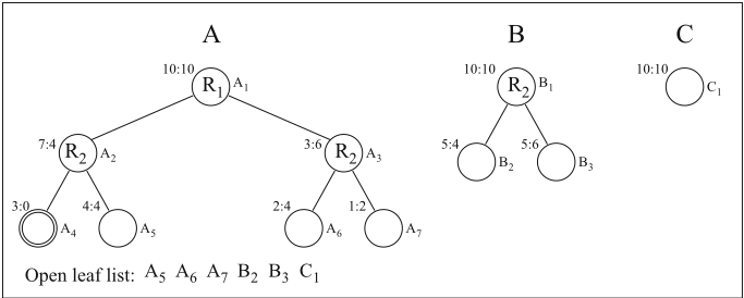
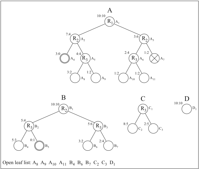
To clarify the forest building procedure, Figures 1 to 3 show three exemplary stages of forest construction, with the trees designated by letters, and internal nodes marked with an identifier corresponding to the rule that split them. Nodes are described by the tree designation followed by a numeric identifier. The training data consists of 20 instances, 10 each of two classes. The class distribution at each node is given to the node's left. For simplicity we assume that MRC is set to one, i.e. splitting is done immediately, if possible at all. We also assume that full rules (not prefixes) lead to the highest information-gain in all cases.
Figure 1 shows the state of the forest after the first rule, Rule R1, has been added. Initially, the root node of Tree A, A1, was the only node on the Open Leaf List. Now, A1 has been split, and two leaves A2 and A3 created. A2, A3 and the root node of Tree B, B1 have been added to the Open Leaf list and A1 has been removed from the list.
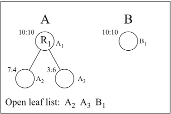
Figure 2 shows the state of the forest after another rule, R2 has been processed. Both A2 and A3 have been split, B1 has been split, and most of the new leaves thus created (A5 through A7 and B2 through B3), along with the root node of Tree C, C1, have been added to the Open Leaf list. A4 now contains instances of only one class (denoted by the double circle) and so was not added to the Open Leaf list, and will not be split any further.
Figure 3 shows the state of the forest after the third rule R3 has been processed. Nodes A5 and A6 have been split, adding A8 through A11 to the Open Leaf list. Node A7 has not been split by R3, and therefore had its Fail count incremented. We set the maximum fail count to 1 (to keep this example concise), and thus A7 (marked by the crossed circle) will now be removed from the Open Leaf list and will not be split any further. A7 will predict a class distribution of (1/3, 2/3) for test examples. Nodes B2 and B3 have been split, producing B4 through B7, of which B4, B6 and B7 will be added to the Open Leaf list, while B5 will not, as it is class-pure. C1 has been split, producing C2 and C3, and the root of tree D, D1, has also been added to the Open Leaf list.
To summarize, R4 F differs from FORF [Assche et al., 2006], in two main ways. First of all FORF does not use full rules in every node, but in contrast pathes from the root to each leaf comprise rules. As logical variables can only be shared across positive pathes, this complicates both generation as well as interpretation of such trees. Like Breiman's original random forest, FORF randomly restricts the set of possible tests (features) and then picks the best test from that restricted set. R4 F on the other hand uses a fully selfcontained randomly generated relational rule as a test. As a consequence, R4 F can easily generate its trees in a staggered parallel fashion, with each new rule being available for all open leaves, while FORF processes both nodes and trees fully sequentially. Even though in theory FORF could also parallelize node and tree generation, it could still not share the expensive cover computation across nodes or trees the way R4 F can.
R4 F can also be seen as an example of dynamic propositionalization [Landwehr et al., 2006], in that the features are generated dynamically on-demand, and do not have to be precomputed in advance as would be common in static propositionalization [Kramer et al., 2000].
2.3 Complexity of Forest Construction
When R4 F generates and evaluates a rule, it then applies the derived test at every open leaf in each active tree. The cost of rule evaluation is the same as for previous uses of Random Relational Rules [Botta et al., 2003; Anderson and Pfahringer, 2007]. As each test is applied to all open leaves, the number of rules required to be evaluated is substantially less than would be required if a new rule were being evaluated for each open leaf, as in standard random forests. The number of rules required for forest construction is heavily influenced by the number of trees in the forest and the Maximum Rule Count. A rough estimate for this value is the sum of the average number of rules required to construct a single tree and the number of trees in the forest, as when the last tree in the forest is completed, the previous trees are also likely to be complete:
where n is the number of trees in the forest and s is the average number of rules required to construct a single tree. Empirical evidence confirming Equation 1 can be found in [Anderson, 2009].
Because of the staggered fashion in which the trees are generated, each tree has access to at least one more rule than its immediate successor and so its construction has probably already finished at the time the construction of that successor finishes. Thus, when the final tree is complete, it is likely that all previous trees are complete or nearly so.
The number of rules required to construct a single tree can vary substantially. It is a function of the particular dataset, the Maximum Rule Count and the particular random rules generated. A worst case upper bound is given by:
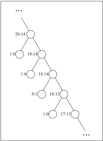
where t is the size of the training set and MRC is the Maximum Rule Count. It is unlikely that this upper bound would be reached under normal circumstances, as it describes the pathological case where each node in the tree is split only after the maximum possible number of rules have been generated, and at every node the split has resulted in one singleinstance leaf and one leaf containing all the remaining instances (see Figure 4). In practice the number of rules required has always been substantially lower than this worst case upper bound.
3 Empirical Evaluation
R4 F was tested using the following standard ILP datasets: Mutagenesis (with and without regression-unfriendly instances) [Srinivasan et al., 1994], Musk1 [Dietterich et al., 1997], Carcinogenesis [Srinivasan et al., 1997], and Diterpenes [Dzeroski et al., 1997]. Mutagenesis and Carcinogenesis were limited to low-level structural information as represented by atoms and bonds; additional propositional information such as global properties lumo or logP , or predefined functional groups was deliberately excluded: they are known to improve classification accuracy significantly, thereby potentially masking the relational performance of the investigated algorithms. The current implementation of R4 F is limited to two classes, so the Diterpenes dataset was transformed into three two-class versions by using all pairwise combinations of the three largest classes called 3, 52 and 54 - Diterpenes54,3, Diterpenes52,3 and Diterpenes52,54.
| Dataset | R4 F | Static | Significant |
|---|---|---|---|
| Carcinogenesis | 61.24 | 60.91 | no |
| Diterpenes52,3 | 97.31 | 96.97 | yes |
| Diterpenes52,54 | 96.24 | 94.22 | yes |
| Diterpenes54,3 | 98.43 | 97.69 | yes |
| Musk1 | 85.32 | 89.13 | no |
| MutagenesisAll | 79.27 | 76.66 | no |
| MutagenesisRF | 85.99 | 84.95 | no |
All results were obtained as averages over ten times tenfold cross-validation. Table 1 compares the accuracy obtained for each dataset, using both R4 F using 500 trees, bagged roots, and MRC equal to 50, and a static propositionalization based on 1000 non-trivial random rules turned into boolean features and processed by an equivalent standard Random Forest.
R4 F has several advantages over a static two-stage method that generates a propositional representation of the data first, and then constructs a Random Forest based on the propositionalized data. The latter approach must generate a sufficiently large number of rules in the first stage without knowing which ones will actually be useful. The propositional representation is potentially very large, but might still not be a good enough approximation of the relational problem. Thus the number of rules to generate will be a critical parameter for the user to set. R4 F on the other hand has a simple stopping condition: completion of the forest, so it never generates more rules than needed. No memory is needed for any intermediate representation, and forest generation is fully parallel. Still, as can be seen in this table, static propositionalization works fairly well for the datasets studied here, and even outperforms R4F on the Musk dataset, even though that win is not statistically significant due to the small size of that dataset. The only significant differences are the wins for R4F on each of the three Diterpenes datasets, in all other cases the standard deviations over the ten times ten-fold crossvalidation runs are too large.
For comparison with published results for FORF[Assche et al., 2006], we also tested R4 F on MutagenesisAll (Table 2) and the Financial dataset (Table 3) using out-of-bag evaluation rather than cross-validation. This was necessary as apparently it is not feasible to evaluate FORF using ten times ten-fold cross-validation. In their paper they used only four datasets, two of which are used here as well, and two were dropped for the following reasons: one is simply too small for any meaningful comparison, as it only comprises 20 examples in total; the other one is a multiple classes problem that the current version of R4 F cannot handle yet. We compare to the highest FORF results listed in their paper, and see that R4 F significantly beats the standard aggregate-less FORF both times. Remember that R4 F currently does not include aggregates, still it is as good as the all FORF-plus-aggregates variants (FORF-LA: lookahead aggregates, FORF-SA: simple aggregates, and FORF-RA: refined aggregates) on one of the two datasets. Clearly, for the second dataset aggregates are essential for near-perfect prediction. Adding aggregates to R4 F will be one major direction for future research.
| Algorithm | Accuracy | ||
|---|---|---|---|
| R4 F | 79.1±1.1 | R4 F is | Significance |
| FORF | 74.7±1.4 | better | 95% |
| FORF-SA | 78.9±1.8 | equal | < 90% |
| FORF-RA | 78.1±1.2 | equal | < 90% |
| FORF-LA | 79.0±1.4 | equal | < 90% |
| Algorithm | Accuracy | ||
|---|---|---|---|
| R4 F | 87.8±0.7 | R4 F is | Significance |
| FORF | 85.7±0.6 | better | 95% |
| FORF-SA | 99.8±0.2 | worse | 99% |
| FORF-RA | 99.7±0.4 | worse | 99% |
| FORF-LA | 99.8±0.4 | worse | 99% |
In addition to measuring accuracy we have also conducted studies to judge the sensitivity of the algorithm to parameter settings and to alternative split rule selection methods. For lack of space we can only summarize here, claiming that, as expected, larger number of trees consistently produce higher accuracies, but that after a couple of hundred trees accuracy usually levels out on a plateau. The MRC or maximum rule count is more of an optimization parameter, usually with optimal values between 50 and 100, where lower values tend to underfit, and higher values cause overfitting. Measuring tree sizes and tree diversity, fully random trees are usually larger and more diverse, and higher MRC values reduce both the size and diversity of trees. For a lot more detail on these aspects please see [Anderson, 2009].
4 Summary and FutureWork
The efficiency and effectiveness of the R4 F algorithm is the result of the application of randomly generated relational rules to the random forests framework. Staggered root initialization allows R4 F to produce diverse trees in parallel, and the experimental results obtained are very competitive with those achieved by another Relational Random Forest algorithm. The main direction for future work will be the inclusion of aggregates into R4 F: FORF benefits significantly from adding aggregates, so R4 F might also be able to take advantage of the additional expressiveness that aggregates provide. As it currently stands, R4 F outperforms the non-aggregate version of FORF and is already equal in performance to the aggregate-enhanced version of FORF on some datasets. Alternative and more targeted random rule generation methods, which work on explicit seed examples that must be covered by a rule, will also be investigated.
@inproceedings{ijcai2009p167,
  title     = {Relational Random Forests Based on Random Relational Rules},
  author    = {Anderson, Grant and Pfahringer, Bernhard},
  booktitle = {Proceedings of the Twenty-First International Joint Conference on
               Artificial Intelligence, {IJCAI-09}},
  publisher = {International Joint Conferences on Artificial Intelligence},
  editor    = {Craig Boutilier},
  pages     = {986--990},
  year      = {2009},
  url       = {https://ijcai.org/proceedings/2009/167},
}
TY - CPAPER TI - Relational Random Forests Based on Random Relational Rules AU - Anderson, Grant AU - Pfahringer, Bernhard T2 - Proceedings of the Twenty-First International Joint Conference on Artificial Intelligence, IJCAI-09 PB - International Joint Conferences on Artificial Intelligence PY - 2009 SP - 986 EP - 990 UR - https://ijcai.org/proceedings/2009/167 ER -Copied
Machine-readable versions of this paper, for tools and AI agents:





