
Combining RCC-8 with Qualitative Direction Calculi: Algorithms and Complexity
Proceedings of the Twenty-First International Joint Conference on Artificial Intelligence. Pages 854-858.
© 2009 International Joint Conferences on Artificial Intelligence
Abstract
Increasing the expressiveness of qualitative spatial calculi is an essential step towards meeting the requirements of applications. This can be achieved by combining existing calculi in a way that we can express spatial information using relations from both calculi. The great challenge is to develop reasoning algorithms that are correct and complete when reasoning over the combined information. Previous work has mainly studied cases where the interaction between the combined calculi was small, or where one of the two calculi was very simple. In this paper we tackle the important combination of topological and directional information for extended spatial objects. We combine some of the best known calculi in qualitative spatial reasoning (QSR), the RCC8 algebra for representing topological information, and the Rectangle Algebra (RA) and the Cardinal Direction Calculus (CDC) for directional information. Although CDC is more expressive than RA, reasoning with CDC is of the same order as reasoning with RA. We show that reasoning with basic RCC8 and basic RA relations is in P, but reasoning with basic RCC8 and basic CDC relations is NP-Complete.Weiming Liu, Li Sanjiang, Renz Jochen
- [Allen, 1983] J.F. Allen. Maintaining knowledge about tem- poral intervals. C. ACM, 26:832-843, 1983.
- [Balbiani et al., 1999] P. Balbiani, J.-F. Condotta, and L. Fariñas del Cerro. A new tractable subclass of the rect- angle algebra. In IJCAI-99, pages 442-447, 1999. IJCAI
- [Cohn and Renz, 2007] A.G. Cohn and J. Renz. Qualitative spatial reasoning. In Frank van Harmelen, Vladimir Lifs- chitz, and Bruce Porter, editors, Handbook of Knowledge Representation. Elsevier, 2007.
- [Gerevini and Renz, 2002] A. Gerevini and J. Renz. Com- bining topological and size information for spatial reason- ing. Artificial Intelligence, 137(1-2):1-42, 2002.
- [Goyal and Egenhofer, 2001] R. Goyal and M.J. Egenhofer. Similarity of cardinal directions. In SSTD, pages 36-58, 2001.
- [Li, 2006] S. Li. On topological consistency and realization. Constraints, 11(1):31-51, 2006.
- [Li, 2007] S. Li. Combining topological and directional in- formation for spatial reasoning. In M.M. Veloso, editor, IJCAI, pages 435-440, 2007. IJCAI
- [Randell et al., 1992] D.A. Randell, Z. Cui, and A.G. Cohn. A spatial logic based on regions and connection. In KR-92, pages 165-176, 1992.
- [Skiadopoulos and Koubarakis, 2005] S. Skiadopoulos and M. Koubarakis. On the consistency of cardinal direction constraints. Artificial Intelligence, 163(1):91-135, 2005.
- [Zhang et al., 2008] X. Zhang, W. Liu, S. Li, and M. Ying. Reasoning with cardinal directions: An efficient algo- rithm. In D. Fox and C.P. Gomes, editors, AAAI, pages 387-392. AAAI Press, 2008.
References were extracted automatically from the PDF and may contain errors.
Full text extracted automatically from the PDF; figures, tables and equations may differ. The PDF is the version of record.
1 Introduction
Qualitative Spatial Reasoning (QSR) is a multi-disciplinary research field that aims at establishing expressive representation formalisms of qualitative spatial knowledge and providing effective reasoning mechanisms. QSR has developed in the last two decades, and dozens of models have been proposed [Cohn and Renz, 2007]. Most of the models focus on single aspect of space, e.g. topology, direction, or shape. This is one major shortcoming of the current QSR formalisms, since many potential applications require multiple aspects.
This paper aims at alleviating this weakness by solving spatial constraints concerning topology and direction, as they
∗This work was partially supported by NSFC (60673105,60621062), and a 973 Program (2007CB311003). The work of S. Li was also partially supported by a Microsoft Research Professorship.
†Corresponding author. Email:lisj@it.uts.edu.au
are two of the most important aspects of space. More specially, we confine ourselves to the combination of topological and directional constraints over extended planner regions, which are closed, regular and bounded, may have multiple pieces or even holes. We adopt the RCC8 algebra [Randell et al., 1992] to express topological constraints, which is one of the most influential formalism for topological relations. As for directional relations, there are two wellknown formalisms that can cope with extended objects, the Rectangle Algebra [Balbiani et al., 1999] and the Cardinal Direction Calculus (CDC) [Goyal and Egenhofer, 2001; Skiadopoulos and Koubarakis, 2005]. RA approximates both the reference and the primary object by their minimum bounding rectangles (MBRs), and relates them by the interval relations between the projected intervals. On the other hand, CDC only approximates the reference object by its MBR, leaving the primary object unchanged. Reasoning with basic CDC constraints is still tractable [Zhang et al., 2008].
Combining spatial constraints of different calculi is a very important problem in QSR. Given a network Θ of topological (RCC8) constraints, and a network Δ of directional (RA or CDC) constraints over the same variables of Θ, the joint satisfaction problem (JSP) is to decide when the joint network Θ ⊎ Δ is satisfiable. Note that we use ⊎, instead of ∪, to indicate that Θ and Δ involve the same variables.
Since topological and directional information is not independent, Θ ⊎ Δ may be unsatisfiable despite both Θ and Δ being satisfiable. Solving the joint satisfaction problem is at least as hard as solving the separate satisfaction problem, which means JSP is NP-hard. In this paper, we only consider basic RCC8 constraints and basic RA or CDC constraints. Since arbitrary constraints can always be backtracked to basic constraints, this does not restrict the usefulness of our results.
We show that the JSP over basic RCC8 and basic RA networks can be solved in polynomial time. We also prove that, the JSP over basic RCC8 and basic CDC networks is NPComplete, by reducing the 3SAT problem to it and devising an exponential decision algorithm.
The rest of this paper proceeds as follows. Section 2 introduces basic notions and related qualitative calculi, including the RCC8 algebra, the Rectangle Algebra (RA), and the Cardinal Direction Calculus (CDC). Sections 3 and 4 consider the computational complexity of the combination of RCC8 with RA and CDC, respectively. Section 5 is the conclusion.
2 Qualitative calculi
The establishment of a proper qualitative calculus is the key to the success of the qualitative approach to temporal and spatial reasoning. This section introduces basic notions and examples of qualitative calculi.
2.1 Basic notions
Let U be the universe of temporal or spatial entities, and set Rel(U) to be the set of binary relations on U. With the usual relational operations of intersection, union, and complement, Rel(U) is a Boolean algebra. A finite set B of nonempty relations on U is jointly exhaustive and pairwise disjoint (JEPD for short) if any two entities in U are related by one and only one relation in B. Write 〈B〉 for the subalgebra of Rel(U) generated by B. Clearly, relations in B are atoms in the algebra 〈B〉. We call 〈B〉 a qualitative calculus on U, and call relations in B basic relations of the calculus.
A constraint over 〈B〉 has the form xγy, where γ is a relation in 〈B〉. We call xγy a basic constraint if γ is a basic relation in B. An important reasoning problem in a qualitative calculus is to determine the satisfiability or consistency of a network Γ = {viγijvj}ni,j=1 of constraints over 〈B〉, where Γ is satisfiable (or consistent) if there is an instantiation {ai}ni=1 in U such that (ai, aj) ∈ γij holds for all 1 ≤ i, j ≤ n.
Since general constraint networks can be reduced to basic networks by backtracking, we confine ourselves to the consistency of basic networks in this paper.
A basic network Γ = {viγijvj}ni,j=1 is path-consistent if every subnetwork involving at most three variables is consistent. Path-consistency can be determined in cubic time. For a basic network, it is easy to see that consistency implies pathconsistency. The opposite proposition does not always hold, it is true for RCC8 and RA, but not true for CDC.
We use JSP(B1, B2) to denote the basic joint satisfaction problem over B1 and B2. Suppose Θ = {viθijvj}ni,j=1 is a basic constraint network over 〈B1〉, and Δ = {viδijvj}ni,j=1 is a basic constraint network over 〈B2〉 involving the same variables. Then we say Θ ⊎ Δ is an instance of JSP(B1, B2). We say Θ ⊎ Δ is bipath-consistent if Θ and Δ are both pathconsistent and θij ∩ δij ̸= ∅ for any 1 ≤ i, j ≤ n (recall θij and δij are subsets of U×U). Bipath-consistency can be determined in polynomial time [Gerevini and Renz, 2002].
2.2 RCC8 algebra
A plane region (or region) is a nonempty regular closed subset of the real plane. In this paper, we only consider bounded regions, which could have multi-pieces and/or have holes. The relations in Table 1 and the converses of TPP and NTPP form a JEPD set [Randell et al., 1992]. Write Btop for this set, and the RCC8 algebra is generated by Btop.
It is known that, for basic RCC8 networks, pathconsistency implies consistency. A cubic realization algorithm was proposed in [Li, 2006]. Since a similar algorithm will be devised later for the combination cases, we give a short description of this algorithm.
Given a basic RCC8 network Θ = {viθij vj }ni,j=1 , suppose Θ is path-consistent. An ntpp-chain in Θ is defined to be a series of variables vi1 , vi2 , · · · , vik such that vis NTPPvis+1 ∈
| Relation | Symb. | Meaning |
|---|---|---|
| equals disconnected externally connected | EQ DC EC | a = b a ∩ b = ∅ a ∩ b ̸= ∅ ∧ a◦ ∩ b◦ = ∅ |
| partially overlap | PO | a◦ ∩ b◦ ̸= ∅ ∧ a ̸⊆ b ∧ a ̸⊇ b |
| tangential proper part non-tangential proper part | TPP NTPP | a ⊂ b ∧ a ̸⊂ b◦ a ⊂ b◦ |
Θ for all s = 1, · · · , k - 1. The ntpp-level l(i) of a variable vi is defined to be the maximum length of the ntpp chains contained in Θ that ends with vi.
A realization can be constructed as follows. Note that a variable can be interpreted as a bounded region with multiple pieces. We first define for each variable vi a finite set Xi of control points as follows. For each i, introduce a point Pi to vi; if viECvj or viPOvj, then introduce a point Pij to vi; if viTPPvj or viNTPPvj, then put all Xi points into Xj. We then expand each point P in Xi a little to obtain a square s(P). These squares are pairwise disjoint. Then, taking the union of these squares, we obtain an instantiation of bounded regions to these vi. This works for all but the EC and NTPP constraints. Further modifications are needed to cope with these constraints (cf. [Li, 2006], or Section 3 of this paper).
2.3 Interval Algebra and Rectangle Algebra
The interval algebra IA [Allen, 1983] is generated by a set Bint of 13 basic relations between closed intervals (see Table 2). For basic IA constraint networks, path-consistency is sufficient to decide consistency. Moreover, we can construct a canonical solution in the following sense.
| Relation | Symb. | Conv. | Meaning |
|---|---|---|---|
| precedes | p | pi | x+ < y- |
| meets | m | mi | x+ = y- |
| overlaps | o | oi | x- < y- < x+ < y+ |
| starts | s | si | x- = y- < x+ < y+ |
| during | d | di | y- < x- < x+ < y+ |
| finishes | f | fi | y- < x- < x+ = y+ |
| equals | eq | eq | x- = y- < x+ = y+ |
Definition 2.1 (canonical set of intervals). Suppose m = {[m-i ,m+i ]}ni=1 is a set of intervals. Let E(m) be the set of end points of intervals in m. We say m is canonical iff E(m) = [0,M]∩Z, whereM is the largest number in E(m).
For a basic satisfiable IA network, it is not hard to work out the total order of all the end points. Hence we can obtain a canonical solution (by assigning 0 to the first end point, 1 to the second, etc). This gives us the following proposition.
Proposition 2.1. If a basic IA constraint network is satisfiable, then it has a unique canonical solution.
IA can be naturally extended to two-dimensional space. We assume an orthogonal basis in the Euclidean plane, and focus on the rectangles sides of which are parallel to the axes of this basis. For a rectangle r, write Ix(r) and Iy(r) as, resp., the x- and y-projection of r. The basic rectangle relation between two rectangles a, b is α ⊗ β iff (Ix(a), Ix(b)) ∈ α and (Iy(a), Iy(b)) ∈ β, where α, β are two basic IA relations. Apparently, there are 13 × 13 = 169 basic rectangle relations, and we write Brec for this set, i.e., Brec = {α ⊗ β : α, β ∈ Bint}. The Rectangle Algebra (RA) is generated by Brec. The following lemma is straightforward.
Lemma 2.1. Let Δ = {vi(αij ⊗ βij)vj}ni,j=1 be a basic RA network. Then Δ is satisfiable iff its projections Δx = {xiαijxj}ni,j=1 and Δy = {yiβijyj}ni,j=1 are satisfiable IA networks.
We also extend the concept of 'canonical' to RA.
Definition 2.2 (canonical set of rectangles). A set of rectangles {mi}ni=1 is canonical iff its x- and y-projections, {Ix(mi)}ni=1 and {Iy(mi)}ni=1 are canonical sets of intervals.
From Prop. 2.1, clearly each path-consistent basic RA network has a unique canonical solution.
The RA relations can be extended from rectangles to arbitrary bounded regions. For a bounded region b, its minimum bounding rectangle (MBR), denoted by M(b), is defined to be the smallest rectangle containing b. The extended RA relation between two bounded regions a and b is defined to be the RA relation between M(a) andM(b). These extended RA relations are useful for expressing directional information.
2.4 Cardinal Direction Calculus
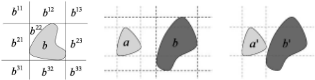
Given a bounded region b in the real plane, by extending the four edges of M(b), we partition the plane into nine tiles, denoted by bij (1 ≤ i, j ≤ 3), see Fig. 1 (left) for illustration.
For a primary region a and a reference region b, the CDC relation of a to b, denoted by δab, is encoded in a 3 × 3 Boolean matrix (dij )1≤i,j≤3, where dij = 1 iff a◦ ∩ bij ̸= ∅ (here a◦ is the interior of a). For example, in Fig. 1 we have
A CDC relation could be any but the zero Boolean matrix, so there are 29 - 1 = 511 basic relations in CDC. We denote this set by Bcdc. Since only the reference object is approximated, CDC is in general more expressive than the RA.
Definition 2.3. For a pair of basic CDC relation (δ, γ), the x-projective interval relation of (δ, γ), written ιx (δ, γ), is defined to be the union of all IA basic relation α s.t. (Ix(m1), Ix(m2)) ∈ α, where {m1,m2} is a solution of {v1δv2, v2γv1}.
If {v1δv2, v2γv1} is consistent, we can prove that ιx (δ, γ) is either a basic IA relation in {o, s, d, f, eq, oi, si, di, fi} or a non-basic IA relation in {p∪m, pi∪mi}. A similar definition and result holds for the y-direction. For example, from Fig. 1, we have ιx (δab, δba) = p ∪ m, ιy (δab, δba) = d.
We call ι(δ, γ) = ιx (δ, γ) ⊗ ιy (δ, γ) the RA relation induced by (δ, γ). In general, for a basic CDC constraint network Δ = {viδijvj}ni,j=1 , we call ι(Δ) = {viιijvj}ni,j=1 the induced RA constraint network of Δ, where ιij = ι(δij , δji).
We next consider special solutions of CDC networks.
Definition 2.4 (maximal solution). A solution {mi}ni=1 of a CDC constraint network Δ is maximal if m′i ⊆ mi holds for any solution {m′i}ni=1 of Δ with M(mi) = M(m′i ).
Definition 2.5 (regular solution). A solution m = {mi}ni=1 of a CDC constraint network is regular if m is maximal and {M(mi)}ni=1 is a canonical set of rectangles.
Although a basic CDC network may have more than one regular solutions, we have the following lemma.
Lemma 2.2. Suppose Δ is a basic CDC network with a solution {mi}ni=1 . Then there exists a unique regular solution {m′i}ni=1 of Δ s.t. for any i, j the basic RA relation between m′i and m′j is the same as that between mi andmj.
[Zhang et al., 2008] devised a cubic algorithm which determines whether a basic CDC network has a (possibly disconnected) solution, and gives a regular one if possible. Here we review the algorithm as it will be used in Section 4. First, we compute a canonical solution of the induced (possibly nonbasic) RA network, which yields a grid space. Next, we remove the grids that violate some constraints from each rectangle. Third, we check whether what we have obtained is a valid solution. In the following, we give a detailed description with a running example illustrated in Table 3 and Fig. 2.
| δij | δji | ιxij ⊗ ιyij | ρxij ⊗ ρyij | |||||
|---|---|---|---|---|---|---|---|---|
| (1, 2) | [0 1 | 0 1 | 0 0 ] | [0 0 | 1 1 | 1 1 ] | o ⊗ o | o ⊗ o |
| 1 | 0 | 0 | 0 | 0 | 0 | |||
| (1, 3) | 1 | 0 0 | 0 0 ] | [0 0 | 0 1 | 0 0 ] | (m∪ p) ⊗fi | p⊗fi |
| [0 1 | 0 | 0 | 0 | 0 | 0 | |||
| (2, 3) | [1 1 | 1 0 | 0 0 ] | [0 0 | 0 0 | 0 1 ] | o ⊗ oi | o ⊗ oi |
| 0 | 0 | 0 | 0 | 1 | 1 | |||
Step 1. Compute the induced RA network Γ0 of Δ. Step 2. Refine Γ0 to a basic RA network Γ = {vi(ρxij ⊗ ρyij )vj}ni,j=1 by setting ρxij = ιxij \(m ∪ mi) and ρyij = ιyij \(m ∪ mi). If Γ is unsatisfiable, then it can be proven that neither is Δ. Suppose Γ is satisfiable and calculate its canonical solution mΓ = {mΓi }ni=1 (cf. Fig. 2 left).

Step 3. This step tries to find a solution m = {mi}ni=1 s.t. M(mi) =M(mΓi ). Recall a basic CDC relation δij is represented as a 3×3 Boolean matrix ((δij )xy). If m is a solution, m◦i ∩ (mj)xy = ∅ holds for any (δij)xy = 0, where (mj)xy is one of the nine tiles generated byM(mj) (cf. Fig. 1). This means, to make m a solution to Δ, we need to exclude all impossible grids frommΓi . Set Ti = ⋃{(mΓj )xy : (δij)xy = 0}nj=1 . Let mi be the closure of mΓi \ Ti (cf. Fig. 2 left). Step 4. Note we may have removed too many tiles so that some constraint like (δij)xy = 1 is violated. The last step then checks whether m = {mi}ni=1 is a solution of Δ. If m is not, we can prove that Δ has no solution at all. Otherwise,
it's not difficult to find out that m is a regular solution.
We need to point out that other regular solutions may exist (cf. Fig. 2 right). We can get all of them by repeating Step 2 to 4 using every possible refinement of Γ0 .
3 Combination of RCC8 and RA networks
We now consider the combination of RCC8 and RA. First we show that bipath-consistency is not sufficient for consistency in JSP(Btop, Brec). Let Γ = {viγijvj}4i,j=1 be the basic RA network as specified in Fig. 3, where mΓ = {mΓi }4i=1 is the canonical solution of Γ. Let Θ = {viθij vj}4i,j=1 be the RCC8 network where θ12 = θ34 = EC and θ13 = θ24 = DC. Although we can verify Θ ⊎ Γ is bipath-consistent, it is not satisfiable. Otherwise, for any solution {mi}4i=1 , we have M(m1) ∩M(m2) =M(m3) ∩M(m4) is a singleton, say P. As θ12 = θ34 = EC, we know P ∈ mi (i = 1, 2, 3, 4), which contradicts θ13 = DC.
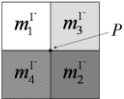
We call point P in the above configuration a conflict point. Definition 3.1 (conflict point). Let Θ be a basic RCC8 network and Γ a basic RA network. Suppose mΓ is the canonical solution of Γ. A point Q is called a conflict point of mΓi if there exists j such that mΓi ∩mΓj = {Q} and θij = EC. We write Ci for the set of all conflict points of mΓi .
Clearly, each conflict point of mΓi is also a corner point of mΓi . This implies that mΓi and mΓj may have at most one common conflict point. Moreover, if m = {mi}ni=1 is a solution of Θ ⊎ Γ s.t. M(mi) = mΓi for all 1 ≤ i ≤ n, then Q ∈ mi. This means Ci ⊂ mi. As a consequence, we have
The following theorem shows that this is also sufficient.
Theorem3.1. SupposeΘ⊎Γ is bipath-consistent. ThenΘ⊎Γ is satisfiable iff Equation 1 holds.
Proof. We only need to show the 'only if' part. Similar to the method for RCC8 alone (cf. Section 2.3 and [Li, 2006]), assuming the ntpp-level l(i) has been computed, we construct a solution m = {mi}ni=1 which also satisfies M(mi) = mΓi . Step 1. Selection of control points For each vi we select a set of control points Xi. First select one point from each edge of mΓi and for Xi. Then, for any j > i with θij = EC or PO, select a point Pij frommΓi ∩ mΓj (which is nonempty because of the bipath-consistency of Θ⊎Γ) for both Xi and Xj. Note that mΓi ∩mΓj could either be a single point, or a line segment, or a rectangle. When choosing Pij from mΓi ∩ mΓj , we should avoid the special points as much as possible in order to make Step 3 simpler. Moreover, the points are required to be distinct if possible. We write P for the set of all the control points.
Step 2. Basic regions associated to control points
For each control point Q, we construct a series of sectors {qi,k : k = 1, · · · , 4}ni=1 and a series of squares {q(i)}ni=1 (see Fig. 4). We call them the basic regions associated to Q. Note that we use an upper case letter to denote a control point, and the corresponding lower case letter (with indices) to denote basic regions. The sectors are chosen in such way as it allows us to distinguish up to four connecting regions in cases where Q is a corner point (such as point P in Fig.3).
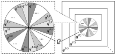
For any two different control points, we require their outermost squares to be disjoint. Furthermore, a basic region must be small enough so that it is not crossed by the border of any mΓi of which Q is not a boundary point. Step 3. Region construction
For each control point Q, set qi = ⋃4k=1 qi,k . Let
Set mi = a4i and m = {mi}ni=1 . It is easy to prove that m satisfies all RCC8 constraints in Θ. To show m also satisfies Γ, we need only prove M(mi) = mΓi for each i. It is clear that a1i and a2i are subsets of mΓi . By the choice of Xi, we know mΓi = M(a1i ) = M(a2i ). If θji = TPP or NTPP, then mΓj ⊆ mΓi by bipath-consistency. This implies M(a3i ) = mΓi . Furthermore, if θji = NTPP, we have (mΓj , mΓi ) ∈ d ⊗ d by bipath-consistency. So for any control point Q in a3j ⊆ mΓj , Q is also in the interior of mΓi . Therefore, by the choice of basic regions, we know the outmost square q(n) at Q, hence q(l(i)) , is contained inmΓi . Therefore, M(a4i ) = mΓi . This proves that m is a solution to Θ⊎Γ.
As a corollary, we have JSP(Btop, Brec) is in P.
Corollary 3.1. For a basic RCC8 network Θ and a basic RA network Γ, consistency of Θ⊎Γ can be decided in cubic time.
Proof. Bipath-consistency of Θ ⊎ Γ can be checked in cubic time. We can construct the unique canonical rectangle solution of Γ in cubic time. The conflict point set Ci can also be computed in cubic time. That is, the condition of Theorem3.1 can be checked in cubic time.
4 Combination of RCC8 and CDC networks
This section discusses the joint satisfaction problem of a basic RCC8 network and a basic CDC network. We first show JSP(Btop, Bcdc) is NP-hard, and then show it is also in NP. Let Θ = {viθijvj}ni,j=1 be a basic RCC8 network and Δ = {viδijvj}ni,j=1 a basic CDC network. Suppose Θ ⊎ Δ is bipath-consistent, and let mΔ = {mΔi }ni=1 be one regular solution of Δ. Clearly, mΔi and mΔj may meet at two or more but finite points (see Fig. 2 for example). These points may introduce conflicts when combined with topological constraints. This is different from RA, where two variables may have at most one conflict point. This will essentially increase the computational complexity.
Lemma 4.1. There is a polynomial reduction from 3SAT to JSP(Btop, Bcdc).
Proof. For each 3SAT instanceϕ = ∧mi=1 (qi1∨qi2∨qi3)with n propositional variables {pk}nk=1 , where qij ∈ {pk}nk=1 ∪ {¬pk}nk=1 , we construct a JSP(Btop, Bcdc) instance Θϕ⊎Δϕ such that ϕ is satisfiable iff Θϕ ⊎Δϕ is consistent. There are three types of spatial variables in Θϕ and Δϕ. Step 1. Grid variables
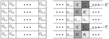
We introduce 10n spatial variables Gij as grid variables, where 1 ≤ i ≤ 2n and 1 ≤ j ≤ 5. The reason we call them 'grid variables' will become clear soon. The CDC constraints between them are specified as in Fig. 5 (left). The RCC8 constraint between Gij,Gi′ j′ is EC if they are 4-neighbors (i.e. {|i - i′ |, |j - j ′ |} = {0, 1}), otherwise DC. These EC constraints make sure that there is no gap between the MBRs of two neighboring grid variables.
Grid variables are mainly used to locate other spatial variables. For a new variable v and a grid variable Gij, we say v occupies Gij if v ∩M(Gij) is nonempty, and its MBR is M(Gij), i.e. M(v ∩M(Gij)) =M(Gij).
Step 2. Spatial variables for propositional variables
For each propositional variable pi in ϕ, four spatial variables Ai,Bi,Ci and Di are introduced. Take Ai as example. By assigning the CDC constraints between Ai and the grid variables, we require Ai occupies G2i-1,1 and G2i-1,4, but has an empty intersection with the interior of the MBR of any other grid variable, see Fig. 5 (right) for illustration, where A+i and A-i are used to denote the two parts of the sketch of Ai. Easy to see, Ai ∩Bi contains at most two points, viz. P + i and P - i , and so does Ci ∩Di.
As for the topological constraints, we set θAj,Bj = θCj ,Dj = EC, and all the others to be DC. The EC constraints imply that both Ai ∩Bi and Ci ∩Di are nonempty. On the other hand, since AiDCCi, we can get the conclusion that Ai and Bi must share only one of P + i and P - i , while Ci and Di share the other one. Step 3. Spatial variables for clauses
For each clause (qj1 ∨qj2 ∨qj3) in ϕ, two new spatial variables Ej and Fj are introduced, both of which occupy three grids. The precise occupied grids are set according to the variables and signs of qjk. One example is given in Fig. 6 to illustrate the construction, where we assume qj1 = pi1 , qj2 = ¬pi2 , qj3 = ¬pi3 . As for the topological constraints, we set θEj ,Fj = EC, while all others (e.g., θAj,Ei ) are DC. This implies Ej ∩ Fj contains at least one point of P - i1 , P + i2 , P + i3 . We assert that it won't be the case that Ai1 ∩Bi1 = {P - i1 }, Ai2 ∩Bi2 = {P + i2 } and Ai3 ∩Bi3 = {P + i3 }. Otherwise, some DC constraint, e.g. that between Ai1 and Ej , will be violated.
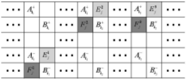
So far we have finished the construction. Next, we show that ϕ is satisfiable iff Θϕ ⊎ Δϕ is consistent.
If Θϕ ⊎Δϕ has a solution m, we can obtain an assignment π : {pi}ni=1 → {true, false} s.t. π(pi) = true iff Ai ∩Bi = {P + i } by m. By Step 3, we can verify that π satisfies ϕ. On the other side, if π is an assignment that satisfies ϕ, we show Θϕ ⊎Δϕ is consistent. The idea is to introduce an instance of JSP(Btop, Brec), in which we have two spatial variables A+i and A-i instead of Ai (also for Bi, Ci, Di), and three variables Ek j (1 ≤ k ≤ 3) instead of Ej (also for Fj). The RA constraints are set according to Fig. 5 and Fig. 6, while the RCC8 constraints are set by Θϕ and π. It can be proved that this new joint network satisfies Eq. 1, and a solution can be obtained in cubic time. A solution of Θϕ ⊎ Δϕ can then be obtained by merging the related regions (e.g. merging A+i and A-i into Ai). The verification is straightforward.
In this way we proved that 3SAT can be reduced to JSP(Btop, Bcdc). The following theorem is clear.
In the remainder of this section, we show JSP(Btop, Bcdc) is also in NP. Let Θ⊎Δ be an instance of JSP(Btop, Bcdc). If Θ⊎Δ is consistent, then it can be proved that Δ has a regular solution (cf. Dfn. 2.5) mΔ = {mΔi }ni=1 and Θ ⊎ Δ has a solution m = {mi}ni=1 such that
- mi ⊆mΔi for each i;
- mi ∩M(g) ̸=∅ for each grid g ⊆mΔi and each i.
If this is the case, we call mΔ a consistent regular solution, and say m is consistent with mΔ. Therefore, to determine whether Θ ⊎ Δ is consistent, we need only check if there exists a consistent regular solution.
Suppose mΔ is a regular solution of Δ. Set
where ∂A is the boundary of A. Set U = ⋃ni=1 Ui. A function f from I = {1, 2, · · · , n} to P(U), i.e. the power set of U, is called a (conflict point) selection function if for any 1 ≤ i, j ≤ n
A consistent regular solution mΔ satisfies:
- edgek (M(mΔi )) ∩mΔi ̸⊆Ni;
- if θij = PO then (mΔi ∩mΔj )◦ ̸= ∅;
- there exists a selection function f : I →P(U),
where edgek (r) returns the k-th edge of a rectangle r (1 ≤ k ≤ 4). The first two conditions are easy to check. As for the third, suppose m is a solution of Θ⊎Δ that is consistent with mΔ. Define f(i) = mi ∩ Ui. It is straightforward to check that f is a selection function.
On the other hand, suppose mΔ is a regular solution of Δ that satisfies the above three conditions. Then we can construct a solution of Θ ⊎ Δ that is consistent with mΔ. This process is similar to that used in JSP(Btop, Brec). We include each point in f(i) into the control points set Xi. Besides, for every variable vi, we select a control point from each grid in mΔi . The process is polynomial. Note that the cardinality of regular solutions of Δ and the cardinality of all possible selection functions f are of order 2n. We have
Together with the NP-hard result, we have
Theorem 4.3. JSP(Btop, Bcdc) is NP-complete.
5 Conclusion
In this paper, we analyzed the interaction between topological and directional constraints for extended spatial regions. We used the rectangle algebra RA and CDC to describe direction information, and RCC8 to express topological constraints. We have shown that the problem of deciding consistency of a joint basic network of RCC8 and RA constraints is still in P, while the one for RCC8 and CDC is NP-Complete.
Our results represent a large step towards the applicability of qualitative spatial reasoning techniques for real-world problems. In particular the result about RCC8 and RA is very promising as it enables efficient reasoning about these two important calculi. It also means that if efficient reasoning is important for a potential application, developers should aim for representing direction information using RA rather than using CDC. Our results about combining RCC8 and CDC are important from a theoretical point of view as they are the first formal results for this combination.
Some related results have been obtained in [Li, 2007], where RCC8 was combined with DIR9, which is a very small sub-algebra of RA that contains only nine basic relations. For a set of directional constraints over DIR9 and a set of topological constraints over a maximal tractable subclass of RCC8, [Li, 2007] proved that the joint satisfaction problem can be reduced to two independent satisfaction problems over RCC8 and RA, respectively. It is worth noting that this work does not restrict constraints to basic ones. While [Li, 2007] shows that reasoning with RCC8 and DIR9 is decidable, it is the present work which proves the decidability of reasoning with RCC8 and the whole RA. Our future work will extend results obtained here to large tractable subclasses of RA and RCC8.
@inproceedings{ijcai2009p146,
  title     = {Combining RCC-8 with Qualitative Direction Calculi: Algorithms and Complexity},
  author    = {Liu, Weiming and Li, Sanjiang and Renz, Jochen},
  booktitle = {Proceedings of the Twenty-First International Joint Conference on
               Artificial Intelligence, {IJCAI-09}},
  publisher = {International Joint Conferences on Artificial Intelligence},
  editor    = {Craig Boutilier},
  pages     = {854--858},
  year      = {2009},
  url       = {https://ijcai.org/proceedings/2009/146},
}
TY - CPAPER TI - Combining RCC-8 with Qualitative Direction Calculi: Algorithms and Complexity AU - Liu, Weiming AU - Li, Sanjiang AU - Renz, Jochen T2 - Proceedings of the Twenty-First International Joint Conference on Artificial Intelligence, IJCAI-09 PB - International Joint Conferences on Artificial Intelligence PY - 2009 SP - 854 EP - 858 UR - https://ijcai.org/proceedings/2009/146 ER -Copied
Machine-readable versions of this paper, for tools and AI agents:





