Answer-Set Programming with Bounded Treewidth

1 Introduction

Over the past decade, Answer-Set Programming (ASP, for short) [Marek and Truszczy´nski, 1999; Niemel¨a, 1999], also known as A-Prolog [Baral, 2002], has become an increasingly acknowledged paradigm for declarative programming. The basic idea of ASP is to encode solutions to a problem into the models of a program in such a way that the solutions are described in terms of rules and constraints. ASP enjoys a large collection of successful applications in the areas of AI and KR showing the potential of this paradigm. However, the underlying complexity of evaluating propositional disjunctive programs (which are the objects we deal with here) shows that the problems ASP has to deal with are highly intractable: the decision problems are located on the second level of the polynomial hierarchy (see [Eiter and Gottlob, 1995]), and the problem of counting all answer sets can analogously be shown to be #NP-complete.

An interesting approach to dealing with such intractable problems is parameterized complexity. In fact, hard problems can become tractable if some problem parameter is bounded by a fixed constant. Such problems are also called fixed-parameter tractable (FPT). One important parameter is treewidth, which measures the "tree-likeness" of a graph. By using a seminal result due to Courcelle [1990], several FPT

∗This work was supported by the Austrian Science Fund (FWF), project P20704-N18.

results in the area of AI and KR have been recently proven tractable by Gottlob et al. [2006], among them also the problem of deciding ASP consistency (i.e. whether a disjunctive logic program has at least one answer set). Treewidth hereby has to be adapted suitably, for instance, by using the incidence graph of the program. However, an FPT result itself does not immediately lead to an efficient algorithm. Indeed, quite some work has been done within the last years to overcome this obstacle. We mention here only some recent results for counting problems: Samer and Szeider [2007] have proposed algorithms for #SAT (counting the number of models of a CNF formula) which follow the principle of dynamic programming; Jakl et al. [2008], on the other hand, map different counting problems to a certain (tractable) datalog fragment. Both approaches have in common that they use the concept of tree-decompositions and proceed by a bottom-up traversal of the tree, such that at each node n, certain information about the subproblem (represented by the subtree rooted at n) is available. Consequently, results for the entire problem can be read off the root of the tree decomposition. Algorithms for counting problems are of particular interest here, since they are closely related to the problem of enumerating solutions, which is, of course, a central requirement in ASP.

In this work, we generalize the dynamic programming approach for #SAT due to Samer and Szeider [2007] to the world of ASP in order to count and enumerate all answer sets of a given program. We thus provide a novel approach for computing answer sets, which significantly differs from standard ASP systems (see [Gebser et al., 2007] for an overview) that usually do not exploit fixed parameter properties. We implemented the proposed method in a prototype system. Our system should not be seen as competitor to general-purpose ASP solvers, but as an alternative for application scenarios where the problems possess low treewidth; usually the ASP encodings then have similarly low treewidth. It is generally believed that many practically relevant problems have low treewidth. Thorup [1998], for instance, shows that the treewidth of the control-flow graph of structured programs (more precisely, goto-free C programs) is at most six. A detailed discussion of applications to which treewidth has been successfully applied is given by Bodlaender [1993].

Results. Our main contributions are as follows.

• An FPT algorithm for deciding ASP consistency in linear time w.r.t. the size of the program.
• An FPT algorithm for counting the number of answer

sets in linear time w.r.t. the size of the program (assuming unit cost for arithmetic operations).

• A novel method for enumerating all answer sets with linear delay.
• Presentation of a first prototype implementation and some preliminary experimental results.

2 Preliminaries

Throughout the paper, we assume a universe U of propositional atoms. A literal is either an atom or a negated atom a. For a set A of atoms, A denotes {a | a ∈ A}. Clauses are sets of literals. An interpretation I is a set of atoms and we define, for a clause c and O ⊆ U, I |=O c iff ((I ∩ O) ∪ (O \ I )) ∩ c ̸= ∅. For a set C of clauses, I |=O C holds iff I |=O c, for each c ∈ C. For O = U, we usually write |= instead of |=O.

Answer-Set Semantics for Logic Programs. A propositional disjunctive logic program (or simply, a program) is a set of rules a1 ∨ · · · ∨ al ← al+1, . . . , am, ¬am+1, . . . , ¬an, (n > 0, n ≥ m ≥ l), where all ai are from U. A rule r of this form consists of a head H(r) = {a1, . . . , al} and a body, given by B+(r) = {al+1, . . . , am} and B-(r) = {am+1, . . . , an}. By At(R) we denote the set of atoms occurring in program R. We often identify a program R with the clause set {H(r)∪B-(r)∪B+(r) | r ∈ R}, and likewise, define the reduct RI of a program R wrt. an interpretation I as {H(r) ∪ B+(r) | B-(r) ∩ I = ∅, r ∈ R}. Following Gelfond and Lifschitz [1991], an interpretation I is an answer set of a program R iff I |= R and for no J ⊂ I, J |= RI . The set of all answer sets of a program R is denoted by AS(R).

Example 2.1 We will use as a running example throughout the paper the program P which consists of the following rules

P has a unique answer set {v, w, x}.

Tree Decomposition and Treewidth. A tree decomposition of a graph G = (V, E) is a pair (T, β), where T is a tree and β maps each node n of T (we use n ∈ T as a shorthand below), to a bag β(n) ⊆ 2V , such that the following conditions are met:

• For each v ∈ V , there is an n ∈ T such that v ∈ β(n).
• For each (v, w) ∈ E. there is an n ∈ T , s.t. v, w ∈ β(n).
• For any three nodes n1, n2, n3 ∈ T, if n2 lies on the path from n1 to n3, then β(n1) ∩ β(n3) ⊆ β(n2).

A tree decomposition (T, β) is called normalized (or nice) [Kloks, 1994] if (i) each node in T has at most two children; (ii) for each node n with two children n1, n2, β(n) = β(n1) = β(n2); and (iii) for each node n with one child n′ , β(n) and β(n′ ) differ in exactly one element.

The width of a tree decomposition is defined as the cardinality of its largest bag β(n) minus one. It is known that every tree decomposition can be normalized in linear time without increasing the width. The treewidth of graph G, denoted as tw(G), is the minimum width over all tree decompositions of G. For arbitrary but fixed w ≥ 1, it is feasible in linear time to decide if a graph has treewidth ≤ w and, if so, to compute a tree decomposition of width w [Bodlaender, 1996].

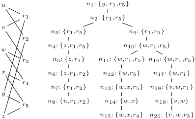
Tree Decompositions of Programs. To build tree decompositions for programs, we shall use incidence graphs. 1 Given a program R, such a graph has as vertices R ∪ At(R), and as edges all pairs (a, r) with an atom a appearing in a rule r of R. In case of normalized tree decompositions, we distinguish between six types of nodes: atom introduction (AI), rule introduction (RI), atom removal (AR), rule removal (RR), branch (B), and leaf (L) nodes. The first four types are usually augmented with the element e (either an atom or rule) which is removed or added compared to the bag of the child node.

Example 2.2 Figure 1 shows the incidence graph GP of program P and a normalized tree decomposition T of GP having width 2. Indeed, we have tw(GP ) = 2, so T has optimal width. Examples for node types are n8 as (L) node, n7 as (u-AR) node, n6 as (z-AI) node, n5 as (r2-RR) node, n4 as (r5-RI) node, and n2 as (B) node.

3 The Dynamic Programming Approach

For this section, let T = (T, β) be a normalized tree decomposition of the incidence graph of a given program R. For M ⊆ R ∪ At(R), we use AM (resp. RM) as a shorthand for At(R) ∩M (resp. R∩M). We refer to the root node of T as rt . For a node n ∈ T , Tn denotes the subtree of T rooted at n. We use A(n) (resp. R(n)) to denote the set of all atoms (resp. rules) which appear in ⋃m∈Tn β(m) (i.e. in some bag of the tree Tn); moreover, A[n] (resp. R[n]) abbreviates A(n) \ β(n) (resp. R(n) \ β(n)), i.e. the set of atoms (resp. rules) which appear only in bags "below" the root of Tn.

We proceed as follows: First, we define the mathematical objects (tree interpretations) which will underly our algorithms. We construct a mapping E(·) from tree interpretations to (standard) interpretations and observe that a certain subset S of the tree interpretations characterizes the answer sets of R. However, we never compute E(·) explicitly. Instead, we define a relation ≺T along the structure of T, in order to efficiently compute S in a bottom-up manner via so-called tree models, a subset of the tree interpretations. Finally, we show how to use this method to count and enumerate the answer sets of program R from a given tree decomposition T for R.

1 See [Samer and Szeider, 2007] for other possible types of graphs and a discussion why incidence graphs are favorable.

3.1 Tree interpretations

Definition 3.1 A tree interpretation for T (T -interpretation, for short) is a tuple (n,M, C) where n ∈ T is a node, M ⊆ β(n) is called assignment, and C ⊆ 2β(n) is called certificate.

The basic intuition behind T -interpretations is as follows: the assignment M of a T -interpretation (n, M, C) contains an interpretation AM over Aβ(n) (implicitly it refers to interpretations I over A(n)) together with rules r ∈ Rβ(n) satisfied by I, i.e. I |=A(n) r. Certificate C can be understood as a set of assignments and carries interpretations (together with satisfied rules in (Rβ(n))I ) which are in a certain subset-relation to M. The following definitions make this more precise.

Definition 3.2 Given n ∈ T and I, J ⊆ A(n), define SATn(I ) = {r | r ∈ R(n), I |=A(n) r} and RSATn(J, I ) = {r | r ∈ R(n) s.t. J |=A(n) r or B-(r) ∩ I ̸= ∅}.

Roughly speaking, SATn(I ) yields those rules of R which occur in bags of the subtree Tn and are satisfied by I. Analogously, RSATn(J, I ) yields such rules which are either satisfied by J or not contained in the reduct RI (thus we can view them as satisfied by J in a trivial way).

Definition 3.3 Let θ = (n,M, C) be a T -interpretation, I ⊆ A(n), and let R∗ = RM ∪ R[n]. We define

Moreover, C is called valid wrt. I in θ, if, for each N ⊆ β(n), it holds that N ∈ C iff there exists J ∈ ren(N, I ) s.t. J ⊂ I.

The rationale behind en(M ) is to yield those extensions of the interpretation AM stored in the assignment M of a T - interpretation θ = (n,M, C) to an interpretation I over A(n) (i.e. over all atoms occurring in bags of Tn), such that the rules RM plus all rules in R[n] (i.e. all rules occurring in bags of Tn, but below n) are satisfied by I. A similar idea is followed by ren(M, I ) which additionally takes the concept of reduct into account.

We are now prepared to define the mapping E(·) and we shall see that for certain T -interpretations θ, E(θ) ⊆ AS(R).

Definition 3.4 For a T -interpretation θ = (n,M, C), let

Definition 3.5 A T -interpretation (n,M, C) is called a root model for T iff n = rt, RM = Rβ(n) and, for each N ∈ C, RN ⊂ RM.

Theorem 3.6 Let Θ be the set of all root models for T . Then, AS(R) = ⋃θ∈Θ E(θ).

Proof. We only show the ⊆-direction. The ⊇-direction is proved analogously. We write Art as shorthand for Aβ(rt) and likewise Rrt for Rβ(rt). Let I ∈ AS(R) and let θ = (rt , M, C) with M = (I∩Art)∪Rrt and C = {N ⊆ β(rt) | ∃J ∈ rert(N, I ) s.t. J ⊂ I}. Note that C is thus valid wrt. I in θ. It remains to show (i) I ∈ ert(M ) and (ii) θ ∈ Θ. (i) holds since RM ∪ R[rt] = Rrt ∪ R[rt] = R, and I |= R

by assumption I ∈ AS(R). For (ii), we have RM = Rrt by definition. We show that for each N ∈ C, RN ⊂ Rrt holds. Suppose this is not the case, i.e. let N ∈ C, such that RN = Rrt . By definition of rert(N, I ), there exists a J ⊂ I, such that for each r ∈ R = Rrt ∪ R[rt], either J |= r or B-(r) ∩ I ̸= ∅. Hence, J |= RI , a contradiction to I ∈ AS(R). ✷

3.2 Tree models

Theorem 3.6 tells us that tree interpretations θ which satisfy E(θ) ̸= ∅ are of particular interest.

Definition 3.7 A T -interpretation θ is called tree model of T (T -model, for short) iff E(θ) ̸= ∅. A T -model that is also a root model for T is called T -root-model.

For leaf nodes n, tree models can be determined as follows. For every M ⊆ β(n), we either have en(M ) = AM in case RM = {r | r ∈ Rβ(n),AM |=Aβ(n) r}, or en(M ) = ∅, otherwise. Hence, to compute all T -models for a leaf node n, one considers each AM ⊆ Aβ(n) and determines RM = {r | r ∈ Rβ(n),AM |=Aβ(n) r}; then AM ∪ RM yields the assignment M for a T -model (n, M, C). Certificate C is given by all J ⊂ AM together with the rules r ∈ Rβ(n), for which either J |=Aβ(n) r or B-(r) ∩AM ̸= ∅ holds.

Example 3.8 Take our example tree-decomposition in Figure 1 and consider leaf node n8. We have β(n8) = {u, r1, r2}. Recall r1 = u ← v, y and r2 = z ← u. We first set u to true. This satisfies r1, i.e. {u} |={u} r1. For the corresponding certificate, there is only one possibility: We set u to false and observe that this satisfies r2. Hence, (n8, {u, r1}, {{r2}}) is a T -model. Another T -model is (n8, {r2}, ∅) and these are the only T -models for n8.

We next define a relation ≺T between T -interpretations. The concrete definition depends on the node type. We first give the definition for the removal and introduction nodes.

Definition 3.9 For T -interpretations θ = (n,M, C) and θ′ = (n′ , M ′ , C ′ ), we have θ′ ≺T θ iff n has a single child n′ , and (depending on the node type of n) the conditions as depicted in the table of Figure 2 are fulfilled. 2

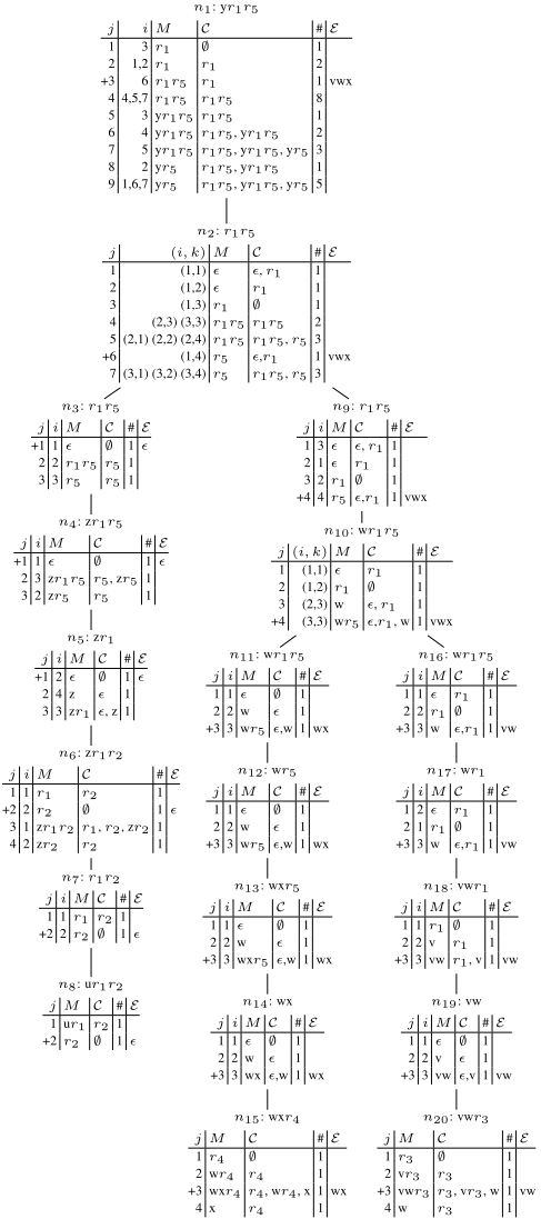
Example 3.10 Recall T -model θ8 = (n8, {u, r1}, {{r2}}). To obtain T -models for n7 (which is a (u-AR) node) from θ8 we have to remove all occurrences of u in θ8, i.e. we get θ8 ≺T (n7, {r1}, {{r2}}) = θ7. Next, we consider n6 which is a (z-AI) node. We have two possibilities. First, we set the new atom z to true, i.e. we get as assignment {z, r1, r2} = {r1} +n6 z (for the definition of operators as +n, see Figure 2). The certificate consists of N1 = {r1} = {r1} ×n6 z, N2 = {z, r2} = {r2} +n6 z and N3 = {r2} = {r2} ×n6 z. Hence, θ7 ≺T (n6, {z, r1, r2}, {N1,N2,N3}) = θ1 6 (also note here that Rz,n6 = ∅). Second, we set the new atom z to false, which yields θ2 6 = (n6, {r1}, {N3}). For the next node n5, which is of type (r2-RR), thus only θ1 6 plays a role since its assignment contains r2 and we obtain θ1 6 ≺T (n5, {z, r1}, {{z}, ∅}) = θ5 (the set {r1} from the certificate of θ1 6 also drops out, since it does not contain r2). Finally, we use θ5 to compute T -models of n4, an (r5-RI)

2 Note that in case n is an (AI)-node, there are two ways how θ′ and θ can be related to each other.

Figure 2: Conditions for (n′ , M ′ , C ′ ) ≺T (n,M, C).

node. We observe that {z, r1, r5} = {z, r1} ⊎n4 r5 since r5 = x ← ¬y, ¬z contains z negated. For the same reason, r5 is added to all sets of the certificate. We obtain θ5 ≺T (n4, {z, r1, r5}, {{z, r5}, {r5}}). We refer already to Figure 4 (which is explained in detail later) to follow this sequence of T -models.

For branch nodes, we partially extend (with a slight abuse of notation) ≺T to a ternary relation as follows.

Definition 3.11 For T -interpretations θ = (n,M, C), θ1 = (n1,M1, C1), θ2 = (n2,M2, C2) we have (θ1, θ2) ≺T θ iff the following conditions hold: (1) n1 and n2 are the two children of n; (2) AM1 = AM2 andM = M1∪M2; (3) C is given by the set (C1 ✶ C2) ∪ ({M1} ✶ C2) ∪ (C1 ✶ {M2}); where C ✶ C ′ is defined as {C ∪C′ | C ∈ C,C′ ∈ C ′ , AC = AC′ }.

Example 3.12 Consider θ′ = (n11, {w, r5}, {∅, {w}}) and θ′′ = (n16, {w}, {∅, {r1}}). Both are T -models. We determine a θ for branch node n10, such that (θ′ , θ′′ ) ≺T θ. Such θ exists (since w is true in the assignment of both θ′ and θ′′ ), and is of the form (n10, {w, r5}, C) with C = {∅, {w}, {r1}} obtained as follows: {∅, {w}} ✶ {∅, {r1}} = {∅, {r1}}; {{w, r5}} ✶ {∅, {r1}} = ∅; {∅, {w}} ✶ {{w}} = {{w}}.

The following lemma is central.

Lemma 3.13 Let θ = (n,M, C) be a T -interpretation. If n is of type (RR), (RI), (AR), or of type (a-AI) and a /∈M, then E(θ) = ⋃θ′≺T θ E(θ′ ). If n is of type (a-AI) and a ∈M, then E(θ) = ⋃θ′≺T θ (E(θ′ ) ∪ {a}). If n is a branch node, then E(θ) = ⋃(θ1,θ2)≺T θ {I1 ∪ I2 | I1 ∈ E(θ1), I2 ∈ E(θ2)}.

Proof (Sketch). Due to space reasons, we only show the case of an (r-RR) node here. The other cases are similar.

In what follows, let n′ be the child of n and M ′ = M ∪{r}. First, note that I ∈ en(M ) iff I ∈ en′ (M ′ ). Indeed, since {r} = R[n] \R[n′ ] = RM′ \RM, RM′ ∪R[n′ ] = RM ∪R[n] and thus SATn(I ) = SATn′ (I ). Similarly, one can show that J ∈ ren(M, I ) iff J ∈ ren′ (M ′ , I ), for any I, J ⊆ A(n).

Let I ∈ E(θ) and θ′ = (n′ , M ′ , C1 ∪ C2), where C1 = {C ∪ {r} | C ∈ C} and C2 = {N ⊆ β(n′ ) | r /∈ N, ∃J ⊂ I s.t. J ∈ ren′ (N, I )}. In fact, θ′ ≺T θ holds. We show I ∈ E(θ′ ). By the observation above, we have I ∈ en′ (M ′ ). To show that C1 ∪ C2 is valid wrt. I in θ′ , suppose it is not the case, i.e. there exists an N ′ ⊆ β(n′ ) such that either N ′ ∈ C1∪C2 or there exists a J ∈ ren′ (N ′ , I ), such that J ⊂ I. By definition of C2, r ∈ N ′ has to hold. We know J ∈ ren(N, I ) iff J ∈ ren′ (N ′ , I ). But then, for N = N ′ \ {r}, either N ∈ C or there exists a J ∈ ren(N, I ), such that J ⊂ I. This yields that C is not valid wrt. I in θ. A contradiction to I ∈ E(θ).

Let I ∈ E(θ′ ) for a θ′ = (n′ , M ′ , C ′ ), such that θ′ ≺T θ. By definition of ≺T , M ′ is of the formM ∪ {r}. Using our previous observation, we get I ∈ en(M ). Since I ∈ E(θ′ ), C ′ is valid wrt. I in θ′ , and we know C = {C \{r} | C ∈ C ′ , r ∈ C}, since θ′ ≺T θ. We show that C is valid wrt. I in θ, which will imply I ∈ E(θ). Again, suppose C is not valid wrt. I in θ, i.e. there exists an N ⊆ β(n), such that either N ∈ C or there exists J ∈ ren(N, I ), such that J ⊂ I. We know that then J ∈ ren′ (N ′ , I ) as well, which is in contradiction to the assumption that C ′ is valid valid wrt. I in θ′ . ✷

Corollary 3.14 Let θ, θ′ , θ′′ be T -interpretations, such that θ′ ≺T θ (resp. (θ′ , θ′′ ) ≺T θ). Then, θ is a T -model iff θ′ is T -model (resp. both θ′ and θ′′ are T -models).

Theorem 3.15 Deciding AS(R) ̸= ∅ can be done in time O(f (w) · |R|), where w denotes the treewidth of R and f is a function that only depends on w but not on R.

Proof (Sketch). Corollary 3.14 suggests the following algorithm: first, we establish the T -models of leaf nodes, then we compute all remaining T -models via ≺T in a bottom-up manner. As soon as we have the T -models for the root node, we check whether they include also a root model for T .

The effort needed for processing a leaf node as well as for the transition from the child node(s) to the parent only depends on the treewidth but not on R. Moreover, the size of T is linearly bounded by the size of R. Hence, this algorithm has the desired time bound. The correctness of this algorithm immediately follows from Theorem 3.6, i.e.: AS(R) ̸= ∅ holds iff there exists at least one T -root-model. ✷

Theorem 3.15 is the desired FPT result for the ASP consistency problem. Indeed, if the treewidth w is bounded by a constant, then AS(R) ̸= ∅ can be decided in linear time.

Example 3.16 The T -models for our running example are depicted in Figure 4, where we grouped them wrt. their nodes and along the structure of the tree of T . T -models which contribute to the single T -root-model (n1, {r1, r2}, {{r1}}) are marked with "+". Following the branches and using the T -models marked with "+", one can see that the used atoms are v, w, x which exactly yields the answer set of our example program P. For illustration, we depict for those T -models θ also the set E(θ) in the last column (as mentioned before, this set is not explicitly computed). Finally, # refers to a function which we define in the next section for counting answer sets.

3.3 Counting and Enumerating Answer Sets

The following observation is important and together with Lemma 3.13 lays the foundation for our counting algorithm.

Proof (Sketch). Suppose to the contrary that there exists an assignment I ∈ E(θ1) ∩ E(θ2). We show that then θ1 = θ2. By definition of E(·), AM1 = AM2 . Moreover, there exists a K ⊆ A[n] such that SATn(AMi ∪K) = RMi ∪ R[n]. By RMi ∩R[n] = ∅ and RM1 ∪R[n] = RM2 ∪R[n] we conclude RM1 = RM2 . Thus M1 = M2. Finally, C1 = {N ⊆ β(n) | ∃J ∈ ren(N, I ), s.t. J ⊆ I} = C2 follows by definition. Hence, θ1 = θ2. ✷

Next, we recursively define a mapping from T -interpretations to numbers.

Definition 3.18 Let θ be a T -interpretation for node n. If θ is not a T -model, let #(θ) = 0, otherwise let

Using Theorem 3.6 and Lemma 3.13 and 3.17, we obtain

Theorem 3.19 Let Θ be the set of all root models of T . Then, |AS(R)| = ∑θ∈Θ #(θ).

Using the same algorithm as sketched in the proof of Theorem 3.15, plus keeping track of the # values for T -models, we immediately obtain the following result.

Theorem 3.20 Assuming unit cost for arithmetic operations, |AS(R)| can be computed in time O(f(w) · |R|), where w = tw(R) and f is a function depending on w but not on R.

For the enumeration problem, we provide in Figure 3 an algorithm which, given a T -root-model θ = (n,M, C), computes the set E(θ) step by step, such that each new element in E(θ) requires only linear delay.

To this end, we consider for a given T -model θ, all θ′ such that θ′ ≺T θ (resp. all (θ′ , θ′′ ) such that (θ′ , θ′′ ) ≺T θ) as stored in an ordered list, and for each such list we use an internal pointer pθ. Function initialize resets all pointers to the first θ′ (resp. to the first pair (θ′ , θ′′ )) in such a list. Function get current(θ) yields the object pθ currently refers to. Function get next(θ) either moves the pointer to the next θ′ (resp. to the next pair (θ′ , θ′′ )) in the list and returns 0; or in case the last element was already reached, it resets pθ to the first element in the list and returns 1. Due to the space restrictions, we cannot discuss the algorithm in detail. However, we note that in general one T -root-model may refer to multiple answer sets. Thus we have to reconstruct all possible such models by traversing the tree downwards - and collect all atoms set to true in at least some assignment - for all possible combinations of T -models related via ≺T .

Function getAS(θ, I, flag)

input: (T -interpretation θ = (n,M, C), interpretation, Boolean) return: (interpretation, Boolean)

begin

if n is leaf-node then return(I, flag); if n is branch node then (θ′ , θ′′ ) = get current(θ); (J, flag ′ ) = getAS(θ′ , I, flag); (K, flag ′′ ) = getAS(θ′′ , J, flag ′ ); else θ′ = (n′ , M ′ , C ′ ) = get current(θ); (K, flag ′′ ) = getAS(θ′ , I, flag); if n is of type (e-AR) and e ∈ M ′ then K = K ∪ {e}; endif if flag ′′ then return (K, get next(θ)); return (K, 0); end Program enumerateAS begin for each T -root-model θ = (rt , M, C) do initialize; repeat (I , flag ) = getAS(θ, AM , 1); output I; until flag; done end

Our ASP algorithm first computes all T -models as sketched in the proof of Theorem 3.15 (within this algorithm, we already keep track of the information used later by the pointers pθ). Then the program enumerateAS iterates through all T -root-models and outputs the corresponding answer sets.

Theorem 3.21 Program enumerateAS works in space O(f (w) · |R|) and outputs all elements in AS(R) with delay O(f (w) · |R|), where w denotes the treewidth of R and f is a function that only depends on w but not on R.

4 Implementation and Results

For our implementation, we have chosen Haskell, a programming language with lazy semantics [Josephs, 1989], thus the desired linear delay is implicit in the evaluation strategy of the language (a computation is only executed when needed). We call our prototype LAPS (lazy answer-set programming system).

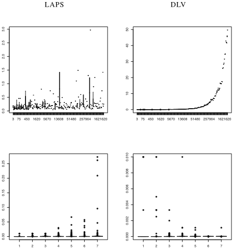
The performance of our straightforward implementation is unprecedented for counting, and is very competitive at low treewidths (up to six) for enumerating the answer sets. Given its early stage of development, LAPS has a high potential for further improvements. We split the evaluation into four steps: (1) parse a disjunctive logic program and generate the data structures for our target language. (2) build the incidence graph of the program and decompose the graph using heuristic methods [Dermaku et al., 2005]. The decomposition is then provided as a data structure for the target language. (3) all parts are merged with the algorithm, compiled and (4) executed. Figure 5 summarizes the runtime behavior of LAPS (assuming the tree decomposition is already given) compared to DLV on a set of randomly generated programs. The first row shows the time required to count the number of answer sets with increasing number of answer sets (here we fixed the treewidth to 5). Clearly DLV's runtime is dependent on the number of answer sets, whereas LAPS' runtime is not affected (excluding time required to handle very large integers). The second row shows the runtime required for enumerating the answer sets (time per answer set) with increasing treewidth. Here, LAPS' runtime increases quickly with larger treewidth whereas DLV even seems to benefit from larger treewidth. The latter effect is due to the fact that our randomly generated programs tend to have more answer sets when the treewidth increases which - in case of DLV - decreases the average cost per answer set. Tests using smodels instead of DLV resulted in a very similar runtime behavior.

5 RelatedWork and Conclusion

Another FPT result for ASP is due to Lin and Zhao [2004], who use the number of cycles in the (directed) dependency graph as parameter. A further interesting parameter here is the number of loops [Ferraris et al., 2006] of a program. We note that programs with an unbounded number of cycles and/or loops can still have low treewidth. Consider P1 = {ai ← ¬bi; bi ← ¬ai | 1 ≤ i ≤ n} or P2 = {an+1 ← a1, ai ← ai+1 | 1 ≤ i ≤ n}. Both have treewidth 2, but the number of cycles (P1), or loops (P2), clearly depends on n.

The work most closely related to ours is by Samer and Szeider [2007], where the #SAT problem in case of bounded treewidth was solved by dynamic programming. We extend their approach to the counting problem (and also the enumeration problem) of ASP. To this end, we have to introduce sophisticated, additional data structures, which ultimately allow us to distinguish between arbitrary and minimal (wrt. to the reduct) models of a given program. Two related problems are constraint satisfaction problems (CSPs) and conjunctive query (CQ) evaluation, for which, apart from treewidth, further methods based on structural decomposition have been used to construct efficient algorithms [Gottlob et al., 2000; Chekuri and Rajaraman, 2000]. These methods usually also work by a bottom-up traversal of a tree structure. As with #SAT, the data propagated up the tree structure is much simpler than in case of ASP solving. On the other hand, the idea of postprocessing by a top-down traversal in order to compute all solutions is also present in the context of CQ evaluation. Recently, dynamic programming has also been applied to logic programming in the context of query answering over Semantic Web data [Ruckhaus et al., 2008]. In this work, dynamic programming is applied to the computation of an optimal join order for CQ evaluation over deductive databases.

To summarize, we introduced in this work novel algorithms for ASP consistency, as well as for counting and enumerating answer sets. The algorithm runs in linear time (resp. with linear delay) if the treewidth of the logic programs is bounded by a constant. Our experiments indicate that this technique may lead to a promising alternative for evaluating ASP programs, if the treewidth remains low. Since tree decompositions of the logic programs are required for the algorithm, our approach will greatly profit from any future progress in the research for efficient tree-decomposition algorithms.

Future research concerns investigations to improve the performance of the proposed method. This includes concepts like balanced and non-normalized tree-decompositions. As well, we plan to study methods for parallelization, which should be easily applicable to the tree-like structure of the required computations. Finally, we want to use lower-level languages (instead of Haskell, where we rely on the compiler to do adequate optimizations automatically) for our algorithms and perform optimizations by hand.

Acknowledgement

We are very grateful to Stefan R¨ummele for valuable comments on a preliminary version of this paper.