
A Soft Global Precedence Constraint
Proceedings of the Twenty-First International Joint Conference on Artificial Intelligence. Pages 566-570.
© 2009 International Joint Conferences on Artificial Intelligence
Abstract
Hard and soft precedence constraints play a key role in many application domains. In telecommunications, one application is the configuration of call control feature subscriptions where the task is to sequence a set of user-selected features subject to a set of hard (catalogue) precedence constraints and a set of soft (user-selected) precedence constraints. When no such consistent sequence exists, the task is to find an optimal relaxation by discarding some features or user precedences. For this purpose, we present the global constraint SOFTPREC. Enforcing Generalized Arc Consistency (GAC) on SOFTPREC is NP-complete. Therefore, we approximate GAC based on domain pruning rules that follow from the semantics of SOFTPREC; this pruning is polynomial. Empirical results demonstrate that the search effort required by SOFTPREC is up to one order of magnitude less than the previously known best CP approach for the feature subscription problem. SOFTPREC is also applicable to other problem domains including minimum cutset problems for which initial experiments confirm the interest.David Lesaint, Deepak Mehta, Barry O'Sullivan, Luis Quesada, Nic Wilson
- [Barták and Čepek, 2008] Roman Barták and Ondrěj Čepek. Incremental filtering algorithms for precedence and depen- dency constraints. IJAIT, 17(1):205-221, 2008.
- [Codish et al., 2008] M. Codish, V. Lagoon, and P. J. Stuckey. Telecommunications feature subscription as a partial order constraint problem. In ICLP, pages 749-753, 2008.
- [Fages and Lal, 2006] Franc ¸ois Fages and Akash Lal. A con- straint programming approach to cutset problems. Com- put. Oper. Res., 33(10):2852-2865, 2006.
- [Garey and Johnson, 1979] M. Garey and D. Johnson. Com- puters and Intractability: A Guide to the Theory of NP- Completeness. W. H. Freeman and Company, 1979.
- [Lesaint et al., 2008a] D. Lesaint, D. Mehta, B. O'Sullivan, L. Quesada, and N. Wilson. Consistency techniques for finding an optimal relaxation of a feature subscription. In ICTAI, pages 283-290, 2008.
- [Lesaint et al., 2008b] D. Lesaint, D. Mehta, B. O'Sullivan, L. Quesada, and N. Wilson. Solving a Telecommunica- tions Feature Subscription Configuration Problem. In CP, pages 67-81, 2008.
- [Rossi et al., 2006] Francesca Rossi, Peter van Beek, and Toby Walsh. Handbook of Constraint Programming. El- sevier Science Inc., 2006.
References were extracted automatically from the PDF and may contain errors.
Full text extracted automatically from the PDF; figures, tables and equations may differ. The PDF is the version of record.
1 Introduction
Precedence constraints play a key role in planning, scheduling and sequencing problems. In internet telephony for instance, service delivery architectures support the sequential activation of call control features. Users can then personalise their call logic by selecting and sequencing features from a catalogue, e.g., announcement followed by call-divert on incoming calls. However, hard constraints apply to avoid undesirable feature interactions, e.g., call-divert and call-waiting are mutually exclusive. This feature subscription configuration problem, which generalises the minimum cutset problem, can be formulated as a constraint optimisation problem [Lesaint et al., 2008b]. Informally, a feature subscription is defined by a set of features, a set of user specified precedence constraints, a function that maps features and user specified precedence constraints to weights, and a set of precedence and exclusion constraints from the catalogue. The task is to find a sequence of features that is consistent with all the constraints. If such a sequence does not exist then the task is to Luis Quesada 4C, UCC, Ireland l.quesada@4c.ucc.ie Nic Wilson 4C, UCC, Ireland n.wilson@4c.ucc.ie find an optimal relaxation of the feature subscription that is closest to the initial requirements of the user. This problem is NP-hard [Lesaint et al., 2008b].
We propose the soft global precedence constraint SOFTPREC that holds if and only if there is a strict partial order on the selected features subject to hard (catalogue) precedence constraints and soft (user-selected) precedence constraints, and the value of the subscription is within the provided bounds. Note that a sequence can be derived from a strict partial order in polynomial time. Enforcing generalised arc consistency (GAC) [Rossi et al., 2006](Chap. 3) on SOFTPREC is NP-complete. Therefore, we approximate it by pruning the domains of the variables based on the rules that follow from the definition of SOFTPREC; this pruning is polynomial. The pruning rules are presented declaratively which allows us to separate concerns. We also present five upper bounds for pruning the bounds of the value of the subscription. These bounds are computed based on the incompatibilities that are inferred between pairs of features, and the dependencies between user precedences and their corresponding features. The tightness of these bounds depends on the degree of inference made on these incompatibilities and dependencies.
We use these bounds along with the other pruning rules of SOFTPREC within branch and bound search to find an optimal relaxation of a feature subscription. We also compare our approach with the alternative constraint programming (CP) approaches presented in [Lesaint et al., 2008b]. Empirical results demonstrate that the filtering achieved by using SOFTPREC reduces the search effort to such an extent that it is up to one order of magnitude faster than the previously known best CP approach for feature subscription problems. We also experiment with minimum cutset problems and compare our approach with the one presented in [Bart´ak and ˇCepek, 2008]. When compared with the latter approach, SOFTPREC reduces the search effort up to two orders of magnitude.
2 Feature Subscription
In this section we provide some background relevant with the feature subscription problem considered in this paper.
Let fi and fj be features, we write a precedence constraint of fi before fj as fi ≺ fj or as 〈fi, fj〉. We write fi ≺≻ fj to mean fi ≺ fj and fj ≺ fi, which corresponds to fi and fj being incompatible (mutually exclusive). A catalogue is a pair 〈F,H〉, where F is a set of features and H is a set of precedence constraints on F. A feature subscription S of a catalogue 〈F,H〉 is a tuple 〈F,H, P,w〉, where F ⊆ F, H is the projection of H on F, i.e., H↓F= {fi ≺ fj ∈ H : {fi, fj} ⊆ F}, P is a set of (user defined) precedence constraints on F , w is a function that maps features and user precedence constraints to weights. The value of S is defined by Value(S) = ∑f∈F w(f ) + ∑p∈P w(p).
A subscription S = 〈F,H, P,w〉 is defined to be consistent if and only if the directed graph 〈F,H ∪ P〉 is acyclic. The time complexity for checking the consistency of a subscription is O(|F| + |H ∪ P|) [Lesaint et al., 2008b]. If a subscription is consistent then there exists at least one sequence of features that respects all the constraints. A relaxation of 〈F,H, P,w〉 is a subscription 〈F ′ ,H′ , P ′ ,w′ 〉 such that F ′ ⊆ F, H′ = H↓F ′ , P ′ ⊆ P↓F ′ , w′ is w restricted to F ′ and P ′ . Let RS be the set of all consistent relaxations of a feature subscription S. We say that Si ∈ RS is an optimal relaxation of S if it has maximum value among all relaxations, i.e., if and only if there does not exist Sj ∈ RS such that Value(Sj) > Value(Si). Finding an optimal relaxation of a subscription is NP-hard [Lesaint et al., 2008b].
A simple constraint optimisation problem (COP) formulation for finding an optimal relaxation of 〈F,H, P,w〉 is as follows. Each feature fi ∈ F is associated with a Boolean variable bf(i) and an integer variable pf(i). The domain of each integer variable pf(i) is {1, . . . , |F|}. Each user precedence constraint (fi ≺ fj) ∈ P is associated with a Boolean variable bp(i, j). A variable v is associated with the objective function. A catalogue precedence constraint, (fi ≺ fj) ∈ H, can be expressed as bf(i) ∧ bf(j) ⇒ (pf(i) < pf(j)). A user precedence constraint (fi ≺ fj) ∈ P can be expressed as bp(i, j) ⇒ (bf(i) ∧ bf(j) ∧ (pf(i) < pf(j))). The objective is to maximise the value of v, where v = ∑fi∈F bf(i) × w(fi) + ∑〈i,j〉∈P bp(i, j) × w(〈i, j〉). Note that this model encodes the precedence relation using absolute position variables. [Lesaint et al., 2008b] present results of using the following consistency techniques: arc consistency (AC), singleton arc consistency (SAC), and restricted singleton arc consistency (RSAC) on the Boolean variables of the model. All these consistency techniques enforce bounds consistency on the objective variable v.
3 The SoftPrec Global Constraint
Let 〈F,H, P, w〉 be a feature subscription. Let bf be a vector of Boolean variables associated with F. We say that fi is included if bf(i) = 1, and fi is excluded if bf(i) = 0. We abuse notation by using bf(i) to mean bf(i) = 1, and ¬bf(i) to mean bf(i) = 0. A similar convention is adopted for the other Boolean variables. Let bp be a matrix of Boolean variables. Here bp is intended to represent a strict partial order on the included features F ′ which is compatible with the catalogue constraints restricted to F ′ .
Definition 1 (SOFTPREC). Let S = 〈F,H, P,w〉 be a feature subscription, bf be a vector of Boolean variables, bp be a matrix of Boolean variables, and v be an integer variable, the global constraint SOFTPREC(S, bf, bp, v) holds if and only if
- bp is a strict partial order restricted to bf, i.e.,
- bp is compatible with H restricted to bf, i.e.,
A solution of SOFTPREC is a consistent relaxation of the subscription 〈F,H, P,w〉. Notice that the minimum cutset problem [Garey and Johnson, 1979] can be expressed in terms of SOFTPREC by associating vertices with features and arcs with catalogue precedence constraints. Therefore, achieving generalised arc consistency on SOFTPREC is NP-hard and hence NP-complete.
If (fi ≺ fj) ∈ H and (fj ≺ fk) ∈ H then fi ≺ fk can be inferred only if fj is included, as features are optional. In order to do this kind of inference we introduce another matrix ψ of auxiliary Boolean variables.
Proposition 1. Let ψ(i, j) ≡ ¬bf(i) ∨ ¬bf(j) ∨ bp(i, j). SOFTPREC(S, bf, bp, v) holds if and only if the following holds:
- bp(i, j) ⇒ bf(i) ∧ bf(j);
- bf(i) ∧ bf(j) ∧ψ(i, j) ⇒¬ψ(j, i);
- bf(j) ∧ψ(i, j) ∧ψ(j, k) ⇒ψ(i, k);
- (fi ≺ fj) ∈ H ⇒ψ(i, j);
- v = Pi∈F bf(i) ×w(i) + P〈i,j〉∈P bp(i, j) ×w(〈i, j〉).
4 Pruning Rules
An algorithm for pruning the domains is presented in terms of rules that follow from the semantics of SOFTPREC. Each pruning rule has the following form: Precondition Postcondition . Here Precondition defines what should be true for the rule to be triggered and Postcondition defines what should be true after executing the pruning rule. The algorithm iterates until no precondition is met.
4.1 Pruning Rules Related to Transitive and Asymmetric Properties
From Proposition 1.1 and the definition of ψ:
bf(i) ∧ bf(j) ∧ ψ(i, j)
bp(i, j)
bp(i, j)
bf(i) ∧ bf(j) ∧ ψ(i, j)
From Proposition 1.2:
bf(i) ∧ ¬bp(i, j) ∧ ψ(i, j)
¬bf(j)
¬bf(i) ∨ ¬bf(j) ∨ ¬ψ(i, j)
¬bp(i, j)
From Proposition 1.3:
From Proposition 1.1, 1.2, and the definition of ψ:
From Proposition 1.4, consistency with the catalogue precedence constraints is ensured by pruning the domain of ψ(i, j) based on the implication (fi ≺ fj) ∈ H ⇒ ψ(i, j).
4.2 Pruning Rules Related to Bounds
Let mv be the maximum value of the subscription, which is defined to be the sum of the weights of all the features and user precedences. Let bv be the backward value of the subscription, which is defined to be the sum of the weights of included features and user precedences. Let bc be the backward cost, which is defined to be the sum of the weights of the excluded features and user precedences.
We say that fi and fj are mutually exclusive when we cannot include both of them, i.e., ψ(i, j) ∧ ψ(j, i). Let M be the set of mutually exclusive pairs of undecided (unassigned) features. Let c+f (i) be the connected cost of including fi, which is defined to be the sum of the weights of the undecided fj and user precedences involving fj such that {fi, fj} ∈ M. Let c-f (i) be the connected cost of excluding fi, which is defined to be the sum of the weight of fi and the weights of the undecided user precedences that involve fi.
Let lb+f (i) and lb-f (i) be the lower bounds on v when fi is included and excluded, respectively. Let ub+f (i) and ub-f (i) be the upper bounds on v when fi is included and excluded, respectively:
We maintain a lower bound, v-, on v and an upper bound, v+, on v. If a bound obtained when excluding (including) fi is not within the bounds of v then fi must be included (excluded).
The upper (lower) bound of v cannot be greater (less) than the maximum (minimum) of the upper (lower) bound of the value resulting from the inclusion and exclusion of fi:
Let v+ p (〈i, j〉) be the connected value of including a user precedence 〈i, j〉 ∈ P, which is defined to be the sum of the weights of the user precedence and the features involved in it (if the latter are undecided). Let c+p (〈i, j〉) be the connected cost of including 〈i, j〉 ∈ P, which is defined to be the sum of the weights of the undecided fk and user precedences involving fk such that either {fi, fk} ∈ M or {fj , fk} ∈ M.
Let lb+p (ρ) and lb-p (ρ) be the lower bounds on v and let ub+p (ρ) and ub-p (ρ) be the upper bounds on v when a user precedence ρ is included and excluded, respectively.
The pruning rules associated with these bounds are obtained by replacing lb+f (i), lb-f (i), ub+f (i), ub-f (i) and bf(i) with lb+p (ρ), lb-p (ρ), ub+p (ρ), ub-p (ρ) and bp(ρ), respectively, in Equations (1) and (2).
If n is the sum of the number of features and user precedences then the worst-case time complexity of the pruning rules presented in this section is O(n3 ) [Lesaint et al., 2008a].
5 Tighter Upper Bounds using Forward Costs
In this section, we introduce the notion of forward cost and use it to compute tighter upper bounds on v when a feature (and a user precedence) is included/excluded.
5.1 Forward Costs
The set of pairs of incompatible features, M, can be associated with an undirected graph where the vertices represent features involved in the incompatibilities and edges represent incompatibilities. Let C1, . . . ,Ck be the components (maximal connected subgraphs) of the graph M. The features involved in any intersecting pairs of incompatible features are always in the same component, e.g. if {fi, fj} ∈ M and {fj, fk} ∈ M then fi, fj and fk are in the same component. If fi ∈ F is not involved in any pair of incompatible features of M, then fi is not in any component.
Let us assume that F = {a, b, c, d, g, h, j}, P = {p, q, r}. Here p, q and r are user precedences defined on features a and b, c and g, and g and j, respectively. Let us also assume that M = {{a, b}, {b, c}, {c, d}, {g, h}}. There are two components of the graph associated with M, which are C1 = {a, b, c, d} and C2 = {g, h}. This is pictorially depicted in Figure 1. An ellipse represents a feature, and the integer number its weight. A dashed line denotes a user precedence between the corresponding features and the integer number its weight. A solid line represents incompatibility between two features based on the set M. The features involved in the components of M are encapsulated in the boxes. Notice that feature j is not involved in any pair of incompatible features of M, therefore, it is not in any component of M.
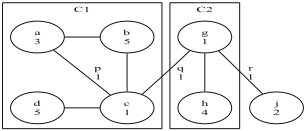
Given the components of M, the forward cost is the sum of the lower-bounds of the costs incurred from the components. We present different forward costs and explain them with an example as illustrated in Figure 1. As the forward cost depends on M, we use the notation fcl (M) to denote the lth forward cost.
The simplest way of computing the forward cost is by computing the minimum weight of features of each component and summing up those weights:
This is based on the fact that at least one feature will be removed from each component. For Figure 1, the forward cost based on fc1 is w(c)+w(g), which is equal to 2. Observe that w(c) and w(g) are the minimum weights of features of C1 and C2, respectively.
Let λi be the lower bound on the number of features that should be excluded from Ci in order to break all the incompatibilities. The value of λi for each Ci is implicitly 1 for fc1 . However, a tighter forward cost can be computed by using a stronger λi and summing the λi smallest costs of excluding features of each component. There exist several ways of doing this. However, for this paper, we define λi to be the maximum value of k such that the sum of the degrees of the first k vertices is no more than the number of edges, where the vertices are listed in decreasing order of degree. Based on this, a forward cost can be computed as follows:
Here minj is the function that gives the j th smallest weight. For Figure 1, the forward cost based on fc2 is w(c) +w(a) + w(g), which is 5. Unlike fc1 , λ1 = 2 for C1 and, therefore, the two smallest weights of features are selected from C1 which are w(a) and w(c).
Neither fc1 nor fc2 take advantage of the fact that the exclusion of a feature may also exclude a user precedence. For this purpose, we present fc3 which can be seen as an extension of fc1 . Instead of considering only the minimum weight of the features of each component, fc3 considers the minimum sum of the weight of a feature and the weights of user precedences that involve the feature.
Here interi(f) is the set of user precedences that involve feature f of Ci and feature g of Cj ̸= Ci. The forward cost based on fc3 is 5 for Figure 1. It is the sum of the cost of excluding c from C1, which is w(a)+w(p)+w(q)/2, and the cost of excluding g from C2, which is w(g)+w(q)/2+w(r). Although c and g are in different components, their exclusion costs include the weight of the user precedence q, since excluding c or g would exclude q. In order to ensure that the weights of user precedences involving features of different components are considered only once, the weights are halved. This allows us to compute the cost of each component independently.
The cost of each component in fc3 is based on the minimum cost incurred by excluding only one feature. However, fc4 may consider multiple features along with their user precedences as shown below:
Here, resti(f) is the set of user precedences that involve features f and g such that f is in Ci and g is not in any Cj. The cost of the component C1 based on fc4 is the sum of the costs of excluding features a and c which are w(a) + w(p)/2 and w(c) + w(p)/2 + w(q)/2 respectively. The cost of the component C2 based on fc4 is the cost of excluding feature g which is w(g) +w(q)/2 +w(r). Hence, the forward cost is 8. Notice that the weights of the user precedences that involve features of the same component are not divided by 2 in fc3 . The reason is that the cost of each component is based on the cost of excluding only one feature which is not true for fc4 . Therefore, fc4 also halves the weights of those user precedences that involve features of the same component.
If the value obtained after subtracting the backward cost and the forward cost from the maximum value of the subscription is less than the upper bound of v, then the upper bound can be updated accordingly.
5.2 Tighter Upper Bounds
This section describes the computation of tighter upper bounds on v due to the inclusion/exclusion of a feature based on the notion of forward cost. Remember that these upper bounds also use the connected costs. Therefore, it may not be possible to consider all the pairs of incompatible features of M for the forward cost computation. Let us consider an example. Let M = {{f1, f2}, {f2, f3}, {f3, f4}, {f5, f6}}. The connected cost of including f2 is w(f1) + w(f3). Therefore, all the incompatibilities that involve either f1 or f3 cannot be considered for the forward cost computation. So the forward cost of including f2 would be based on only one pair of incompatible features, which is {f5, f6}. Similarly, the forward cost of excluding f2 would be based on {f3, f4} and {f5, f6} pairs of incompatible features.
Let M + f (i) be the subset of the pairs of features of M based upon which the forward cost of including fi is computed. Formally, M + f (i) = M - {{j, k} ∈ M : {i, j} ∈ M}. Let M - f (i) be the subset of pairs of features of M based upon which the forward cost of excluding fi is computed. Formally, M - f (i) = M - {{i, j} ∈ M}. Based on the forward cost with respect to the sets M + f (i) and M - f (i), the tighter upper bounds can be defined as follows:
The computation of the upper bounds, as presented in Equation (3), could be expensive as its worst-case time complexity is O(n4 ), where n is |F| + |P|. A less expensive approach would be to compute fc(M) and store the cost of each component of M. An under-estimate of the forward cost of including/excluding fi (fc(M + f (i))/fc(M - f (i))) can be computed by subtracting the cost of the component associated with fi from the sum of the cost of all the components of M, i.e., fc(M). By sacrificing some incompatible pairs of features of the component associated with fi, the worst-case time complexity would then be O(n3 ). A similar approach can be used for tightening the upper bounds on v when a user precedence is included/excluded.
6 Comparison of Pruning
We use the notation Φac and Φsac to denote the pruning achieved by enforcing AC and SAC respectively on the Boolean variables of the model, as presented in Section 2. Both Φac and Φsac enforce bounds consistency on the objective variable v. We use the notation Φsp to denote the pruning achieved by using the rules of SOFTPREC. In this section we compare Φac, Φsp, and Φsac. For simplicity, we ignore user precedences. Nevertheless, the results can be extended for user precedences.
Proposition 2. Φsp and Φsac are incomparable.

Figure 3: Φsp > Φsac
Proof. We show that Φsp and Φsac are incomparable by showing cases where each prunes more than the other one. In Figures 2 and 3, a dashed (solid) ellipse represents an undecided (included) feature, and an edge represents a hard precedence constraint. All features have weight equal to 1.
In Figure 2, if v= 3 and v+ = 4, then Φsac determines the undecided variables. Φc includes feature a, since excluding it results in the inclusion of b and c, which causes a failure. As a is included, b is excluded, which causes the inclusion of c. Φsp is not able to include a, since the bounds on v when excluding a are within the bounds of v.
In Figure 3, if v= 0 and v+ = 2 then Φsp updates v+ to 1. This is not done by Φsac since the inclusion/exclusion of each feature does not make the subproblem arc-inconsistent.
Proposition 3. Φsp is tighter than Φac.
Proof. To prove Φsp is tighter than Φac, we show that if Φac includes/excludes a feature or prunes the bounds of v then Φsp also does that, and the converse does not always hold.
Only the sum constraint of Φac can include/exclude a feature. The lower bounds on v when including/excluding fi in Φac are bv + w(i) and bv respectively, which are the same for Φsp. The upper bounds of including/excluding fi in Φac are mv - bc and mv - bc - w(i) respectively, which are greater than or equal to the bounds of Φsp (see Equation (1)). Therefore, each feature included/excluded by Φac is also included/excluded by Φsp, and each value removed from v by Φac is also removed by Φsp.
In order to show that the inclusion/exclusion of a feature by Φsp does not imply the same by Φac, we consider a trivial example. Assume that f1, f2 and f3 are in F and have weight equal to 1, f1 ≺≻ f2, f1 ≺≻ f3 are catalogue constraints, and v- is 2 and v+ is 3. The upper bound on v when including f1 in Φsp would be 1, since f1 is mutually exclusive with f2 and f3. Therefore Φsp would exclude f1. Based on the sum constraint, the upper bound on v when including f1 in Φac would be 3. Therefore, Φac would not exclude f1. Thus, Φsp is tighter than Φac.
7 Experimental Results
In this section, we empirically evaluate the performance of the pruning rules and bounds computation of SOFTPREC.
All the search algorithms were implemented using Choco 1 and were equipped with a static version of the dom/deg variable ordering heuristic, where dom is the domain size and deg is the original degree of a variable. All the experiments were performed on a PC Pentium 4 (CPU 1.8 GHz and 768MB of RAM) processor. The performances of all the approaches are measured in terms of nodes and runtime in seconds.
1 http://choco.sourceforge.net/
| SP 0 | SP 1 | SP 2 | SP 3 | SP 4 | |
|---|---|---|---|---|---|
| time (ms) | 105,240 | 65,539 | 60,689 | 52,735 | 45,720 |
| nodes | 32,880 | 18,111 | 15,272 | 14,052 | 10,143 |
7.1 Feature Subscription Problem
We experimented with a variety of random catalogues and many classes of random feature subscriptions [Lesaint et al., 2008b]. A random catalogue is defined by a tuple 〈nc,mc, Tc〉. Here, nc is the number of features, mc is the number of catalogue precedence constraints and Tc ⊆ {≺, ≻ ,≺≻} is a set of types of constraints. A random feature subscription is defined by a tuple 〈nu,mu,w〉. Here, nu is the number of features, mu is the number of user precedence constraints and w is an integer greater than 0. Each feature and each user precedence constraint is associated with an integer weight which is between 1 and w inclusive.
We generated catalogues of the following forms: 〈50, 250, {≺,≻}〉, 〈50, 500, {≺,≻,≺≻}〉 and 〈50, 750, {≺ ,≻}〉. For each random catalogue, we generated 〈5, 5, 4〉, 〈10, 10, 4〉, . . . , 〈45, 45, 4〉 classes of random feature subscriptions. For each class, 10 instances were generated and their mean results are reported in this paper.
We first investigated the impact of using different upper bounds on v. The notation SP0 is used to denote the computation of the upper bound without any forward cost and SPi, 1 ≤ i ≤ 4, to denote the computation of the upper bound with fci as presented in Section 5. Due to the lack of space, the results of only the hardest problems that we experimented with are shown in Table 1. Notice that without forward cost SOFTPREC visits almost 50%more nodes. The computation of a tight forward cost, as in SP4, pays off by saving time and nodes. In the remainder of this section, the results obtained by using SP4 are denoted by SP.
We also compared the results of SP with the results obtained by maintaining AC, SAC and RSAC on the COP model as presented in Section 2. The results are shown in Table 2. Note that RSAC is known to be the most efficient CP approach for feature subscription problems [Lesaint et al., 2008b]. The results suggest that AC is inferior to the other approaches by several orders of magnitude. Results also suggest that maintaining RSAC on the Boolean variables reduces the number of nodes and time significantly. Note that RSAC usually visits more nodes than those visited by SAC, but the difference between them is not that significant. SP outperforms all the approaches in terms of nodes and time. It spends at least 5 to 11 times less time than RSAC on hard instances.
7.2 MinimumCutset Problem
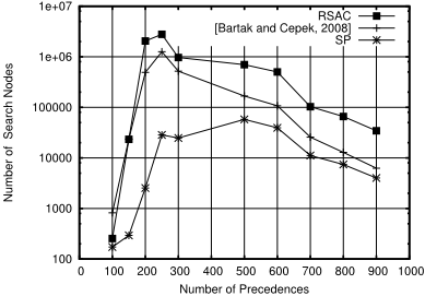
We also demonstrate the efficiency of SOFTPREC on the well known minimum cutset problem [Garey and Johnson, 1979]. The minimum cutset problem consists of only hard precedence constraints and the task is to find the largest set of vertices such that the sub-graph induced by these vertices does not contain a cycle. We use the same instances as those used in [Bart´ak and ˇCepek, 2008] and compare with their approach as well as with RSAC. We remark that when there are no user precedences the approach in [Bart´ak and ˇCepek, 2008] is similar to SP0. Figure 4 shows the results in terms of nodes using a logarithmic scale. Results in terms of time coincide with nodes, but they are not shown due to lack of space. SOFTPREC outperforms both the approaches significantly in terms of nodes and time. When there are 200 precedence constraints, SOFTPREC visits two orders of magnitude fewer nodes when compared with the approach in [Bart´ak and ˇCepek, 2008], and three orders of magnitude fewer nodes when compared with those of RSAC.
| 〈50, 750, {≺, ≻}〉 | 〈50, 500, {≺, ≻, ≺≻}〉 | 〈50, 250, | {≺, ≻}〉 | |||||||||
|---|---|---|---|---|---|---|---|---|---|---|---|---|
| subscription | AC | SAC | RSAC | SP | AC | SAC | RSAC | SP | AC | SAC | RSAC | SP |
| Results in terms of search nodes | ||||||||||||
| 〈30, 30, 4〉 | 100,644 | 655 | 787 | 183 | 17,160 | 143 | 167 | 50 | 104,731 | 230 | 262 | 158 |
| 〈35, 35, 4〉 | 508,318 | 2,008 | 2,366 | 396 | 97,321 | 378 | 451 | 111 | 722,328 | 1,224 | 1,465 | 744 |
| 〈40, 40, 5〉 | 2,209,450 | 5,947 | 6,843 | 993 | 242,609 | 781 | 922 | 188 | 6,155,598 | 9,398 | 11,123 | 2,707 |
| 〈45, 45, 4〉 | 8,055,304 | 16,047 | 18,469 | 2,425 | 740,587 | 1,607 | 1,925 | 428 | 66,905,754 | 31,404 | 37,277 | 10,143 |
| Results in terms of time (in seconds) | ||||||||||||
| 〈30, 30, 4〉 | 24.27 | 3.92 | 3.52 | 0.50 | 2.49 | 0.54 | 0.48 | 0.15 | 20.34 | 1.16 | 1.04 | 0.33 |
| 〈35, 35, 4〉 | 146.72 | 15.01 | 13.68 | 1.52 | 16.18 | 1.82 | 1.69 | 0.44 | 183.49 | 9.13 | 8.70 | 2.16 |
| 〈40, 40, 5〉 | 779.77 | 50.62 | 47.34 | 4.71 | 47.73 | 4.43 | 4.09 | 0.83 | 1,836.39 | 81.77 | 76.59 | 9.46 |
| 〈45, 45, 4〉 | 3,468.08 | 164.83 | 149.36 | 13.86 | 164.89 | 11.03 | 10.19 | 2.26 | 23,009.72 | 345.10 | 320.01 | 45.72 |
8 RelatedWork
[Codish et al., 2008] propose a SAT approach to the feature subscription problem by modeling it as a partial order constraint problem. Although the results reported in [Codish et al., 2008] appear to be better than the results in [Lesaint et al., 2008b], the results of the former were obtained on easier instances. A global constraint for cutset problems is proposed in [Fages and Lal, 2006]. The filtering rules of this global constraint are based on graph contraction operations. We still need to compare SOFTPREC with the cutset constraint.
9 Conclusions and FutureWorks
We proposed the soft global precedence constraint SOFTPREC. Since achieving GAC on SOFTPREC is NP-hard, we presented a set of rules that follow from the semantics of SOFTPREC. The pruning achieved by these rules approximates GAC on SOFTPREC. We introduced the notion of forward cost, and based on it, we proposed various upper bounds computation techniques. We also showed that the pruning achieved by the rules of SOFTPREC is tighter than the pruning achieved by AC on the discussed COP model. The former is incomparable with SAC on the COP model. Empirical results obtained using feature subscription and min-cutset problems demonstrate that SOFTPREC significantly outperforms the other approaches.
In our future work we would like to further investigate tighter bounds. It would also be interesting to investigate the performance of SOFTPREC on other benchmarks.
Acknowledgements
This material is based upon works supported by the Science Foundation Ireland under Grant No. 05/IN/I886, and Embark Post Doctoral Fellowships No. CT1080049908 and No. CT1080049909.
@inproceedings{ijcai2009p100,
  title     = {A Soft Global Precedence Constraint},
  author    = {Lesaint, David and Mehta, Deepak and O'Sullivan, Barry and Quesada, Luis and Wilson, Nic},
  booktitle = {Proceedings of the Twenty-First International Joint Conference on
               Artificial Intelligence, {IJCAI-09}},
  publisher = {International Joint Conferences on Artificial Intelligence},
  editor    = {Craig Boutilier},
  pages     = {566--570},
  year      = {2009},
  url       = {https://ijcai.org/proceedings/2009/100},
}
TY - CPAPER TI - A Soft Global Precedence Constraint AU - Lesaint, David AU - Mehta, Deepak AU - O'Sullivan, Barry AU - Quesada, Luis AU - Wilson, Nic T2 - Proceedings of the Twenty-First International Joint Conference on Artificial Intelligence, IJCAI-09 PB - International Joint Conferences on Artificial Intelligence PY - 2009 SP - 566 EP - 570 UR - https://ijcai.org/proceedings/2009/100 ER -Copied
Machine-readable versions of this paper, for tools and AI agents:





