
Best-First Utility-Guided Search
Proceedings of the Twentieth International Joint Conference on Artificial Intelligence. Pages 2378-2383.
© 2007 International Joint Conferences on Artificial Intelligence
Abstract
In many shortest-path problems of practical interest, insufficient time is available to find a provably optimal solution. One can only hope to achieve a balance between search time and solution cost that respects the user's preferences, expressed as a utility function over time and cost. Current state-of-the-art approaches to this problem rely on anytime algorithms such as Anytime A* or ARA*. These algorithms require the use of extensive training data to compute a termination policy that respects the user's utility function. We propose a more direct approach, called Bugsy, that incorporates the utility function directly into the search, obviating the need for a separate termination policy. Experiments in several challenging problem domains, including sequence alignment and temporal planning, demonstrate that this direct approach can surpass anytime algorithms without requiring expensive performance profiling.
- [Bonet and Geffner, 2001] B. Bonet and H. Geffner. Plan- ning as heuristic search. Artificial Intelligence, 129(1- 2):5-33, 2001.
- [Dechter and Pearl, 1988] Rina Dechter and Judea Pearl. The optimality of A*. In Laveen Kanal and Vipin Kumar, editors, Search in Artificial Intelligence, pages 166-199. Springer-Verlag, 1988. IJCAI-07
- [Hansen et al., 1997] Eric A. Hansen, Shlomo Zilberstein, and Victor A. Danilchenko. Anytime heuristic search: First results. CMPSCI 97-50, University of Massachusetts, Amherst, September 1997.
- [Hart et al., 1968] Peter E. Hart, Nils J. Nilsson, and Bertram Raphael. A formal basis for the heuristic determination of minimum cost paths. IEEE Transactions of Systems Sci- ence and Cybernetics, SSC-4(2):100-107, July 1968.
- [Haslum and Geffner, 2001] Patrik Haslum and Héctor Geffner. Heuristic planning with time and resources. In Proceedings of ECP-01, 2001.
- [Hoffmann and Nebel, 2001] Jörg Hoffmann and Bernhard Nebel. The FF planning system: Fast plan generation through heuristic search. Journal of Artificial Intelligence Research, 14:253-302, 2001.
- [Hohwald et al., 2003] Heath Hohwald, Ignacio Thayer, and Richard E. Korf. Comparing best-first search and dynamic programming for optimal multiple sequence alignment. In Proceedings of IJCAI-03, pages 1239-1245, 2003. IJCAI
- [Kobayashi and Imai, 1998] Hirotada Kobayashi and Hi- roshi Imai. Improvement of the A* algorithm for multiple sequence alignment. In Proceedings of the 9th Workshop on Genome Informatics, pages 120-130, 1998.
- [Korf, 1990] Richard E. Korf. Real-time heuristic search. Ar- tificial Intelligence, 42:189-211, 1990.
- [Likhachev et al., 2004] Maxim Likhachev, Geoff Gordon, and Sebastian Thrun. ARA*: Anytime A* with prov- able bounds on sub-optimality. In Proceedings of NIPS 16, 2004.
- [Nilsson, 1971] Nils J. Nilsson. Problem-Solving Methods in Artificial Intelligence. McGraw-Hill, 1971.
- [Nilsson, 1980] Nils J. Nilsson. Principles of Artificial Intel- ligence. Tioga Publishing Co, 1980.
- [Pearl and Kim, 1982] Judea Pearl and Jin H. Kim. Studies in semi-admissible heuristics. IEEE Transactions on Pat- tern Analysis and Machine Intelligence, PAMI-4(4):391- 399, July 1982.
- [Pohl, 1970] Ira Pohl. Heuristic search viewed as path find- ing in a graph. Artificial Intelligence, 1:193-204, 1970.
- [Russell and Wefald, 1991] Stuart Russell and Eric Wefald. Do the Right Thing: Studies in Limited Rationality. MIT Press, 1991.
- [Zhou and Hansen, 2002] Rong Zhou and Eric A. Hansen. Multiple sequence alignment using Anytime A*. In Pro- ceedings of AAAI-02, pages 975-976, 2002.
- [Zhou and Hansen, 2006] Rong Zhou and Eric Hansen. Breadth-first heuristic search. Artificial Intelligence, 170(4-5):385-408, 2006.
References were extracted automatically from the PDF and may contain errors.
Full text extracted automatically from the PDF; figures, tables and equations may differ. The PDF is the version of record.
1 Introduction
Important tasks as diverse as planning and sequence alignment can be represented as shortest-path problems. If sufficient computation is available, optimal solutions to such problems can be found using A* search with an admissible heuristic [Hart et al., 1968]. However, in many practical scenarios, time is limited or costly and it is not desirable, or even feasible, to look for the least-cost path. Search effort must be carefully allocated in a way that balances the cost of the paths found with the required computation time. This tradeoff is expressed by the user's utility function, which specifies the subjective value of every combination of solution quality and search time. In this paper, we introduce a new shortestpath algorithm called BUGSY that explicitly incorporates the user's utility function and uses it to guide its search.
A* is a best-first search in which the 'open list' of unexplored nodes is sorted by f(n) = g(n) + h(n), where g(n) denotes the cost experienced in reaching a node n from the initial state and h(n) is typically a lower bound on the cost of reaching a solution from n. A* is optimal in the sense that no algorithm that returns an optimal solution using the same lower bound function h(n) visits fewer nodes [Dechter and Pearl, 1988]. However, in many applications solutions are needed faster than A* can provide them. To find a solution faster, it is common practice to increase the weight of h(n) via f(n) = g(n) +w · h(n), with w ≥ 1 [Pohl, 1970]. In the recently proposed ARA* algorithm [Likhachev et al., 2004], this scheme is extended to return a series of solutions of decreasing cost over time. The weight w is initially set to a high value and then decremented by δ after each solution. If allowed to continue, w eventually reaches 1 and the cheapest path is discovered. Of course, finding the optimal solution this way takes longer than simply running A* directly.
These algorithms suffer from two inherent difficulties. First, it is not well understood how to set w or δ to best satisfy the user's needs. Because it is linked to solution cost rather than solving time, it is not clear how to achieve a desired trade-off. Setting w too high or δ too low can result in many poor-quality solutions being returned, wasting time. But if w is set too low or δ too high, the algorithm may take a very long time to find a solution. Therefore, to use a weighted A* technique the user must perform many pilot experiments in each new problem domain to find good parameter settings.
Second, for anytime algorithms such as ARA*, the user must estimate the right time to stop the algorithm. The search process appears as a black box that could emit a significantly better solution at any moment, so one must repeatedly estimate the probability that continuing the computation will be worthwhile according to the user's utility function. This requires substantial prior statistical knowledge of the run-time performance profile of the algorithm and rests on the assumption that such learned knowledge applies to the current instance.
These difficulties point to a more general problem: anytime algorithms must inherently provide suboptimal performance due to their ignorance of the user's utility function. It is simply not possible in general for an algorithm to quickly transform the best solution achievable from scratch in time t into the best solution that would have been achievable given time t + 1. In the worst case, visiting the next-most-promising solution might require starting back at a child of the root node. Without the ability to decide during the search whether a distant solution is worth the expected effort of reaching it, anytime algorithms must be manually engineered according to a policy fixed in advance. Such hardcoded policies mean that there will inevitably be situations in which anytime algorithms will either waste time finding nearby poor-quality solutions or overexert themselves finding a very high quality solution when any would have sufficed.
In this paper we address the fundamental issue: knowledge of the user's utility function. We propose a simple variant of best-first search that represents the user's desires and uses an estimate of this utility as guidance. We call the approach BUGSY (Best-first Utility-Guided Search-Yes!) and show empirically across several domains that it can successfully adapt its behavior to suit the user, sometimes significantly outperforming anytime algorithms. Furthermore, this utility-based methodology is easy to apply, requiring no performance profiling.
2 The BUGSY Approach
Ideally, a rational search agent would evaluate the utility to be gained by each possible node expansion. The utility of an expansion depends on the utility of the eventual outcomes enabled by that expansion, namely the solutions lying below that node. For instance, if there is only one solution in a treestructured space, expanding any node other than the one it lies beneath has no utility (or negative utility if time is costly). We will approximate these true utilities by assuming that the utility of an expansion is merely the utility of the highestutility solution lying below that node.
We will further assume that the user's utility function can be captured in a simple linear form. If f(s) represents the cost of solution s, and t(s) represents the time at which it is returned to the user, then we expect the user to supply three constants: Udefault, representing the utility of returning an empty solution; wf , representing the importance of solution quality; and wt, representing the importance of computation time. The utility of expanding node n is then computed as
where s ranges over the possible solutions available under n. We follow the decision-theoretic tradition of better utilities being more positive, requiring us to subtract the estimated solution cost f(s) and search time t(s). (In the discussion below, this will mean that lower bounds on f(s) and t(s) will yield an upper bound on U(n).) This formulation allows us to express exclusive attention to either cost or time, or any linear trade-off between them. The number of time units that the user is willing to spend to achieve an improvement of one cost unit is wf/wt. This quantity is usually easily elicited from users if it is not already explicit in the application domain. (Of course, such a utility function would also be necessary when constructing the termination policy for an anytime algorithm.) Although superficially similar to weighted A*, BUGSY's node evaluation function differs because wf is applied to both g(n) and h(n).
Of course, the solutions s available under a node are unknown, but we can estimate some of their utilities by using functions analogous to the traditional heuristic function h(n). Instead of merely computing a lower bound on the cost of the cheapest solution under a node, we also compute the lower bound on distance in search nodes to that hypothetical cheapest solution. In many domains, this additional estimate entails only trivial modifications to the usual h function. Search distance can then be multiplied by an estimate of time per expansion to arrive at t(s). (Note that this simple estimation method makes the standard assumption of constant time per node expansion.) To provide a more informed estimate, we can also compute bounds on the cost and time to the nearest solution in addition to the cheapest. Again, standard heuristic functions can often be easily modified to produce this information. U(n) can then be estimated as the maximum of the two utilities. For convenience, we will notate by f(n) and t(n) the values inherited from whichever hypothesized solution had the higher utility.
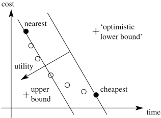
Figure 1 illustrates this computation schematically. The two solid dots represent the solutions hypothesized by the cheapest and nearest heuristic functions. The dashed circles represent other possible solutions, demonstrating a trade-off between those two extremes. The dotted lines represent contours of constant utility and the dotted arrow shows the direction of the utility gradient. Assuming that the two solid dots represent lower bounds, then an upper bound on utility would combine the cost of the cheapest solution with the time to the nearest solution. However, this is probably a significant overestimate. 1 Note that under different utility functions (different slopes for the dotted lines) the relative superiority of the nearest and cheapest solutions can change.
2.1 Implementation
Figure 2 gives a pseudo-code sketch of a BUGSY implementation. The algorithm closely follows a standard best-first search. U(n) is an estimate, not a true upper bound, so it can underestimate or change arbitrarily along a path. This implies that we might discover a better route to a previously expanded state. Duplicate paths to the same search state are detected in steps 7 and 10; only the cheaper path is retained. We record links to a node's children as well as the preferred parent so that the utility of descendants can be recomputed
1 It is interesting to note that taking the time of the cheapest and the cost of the nearest is not a true lower bound on utility because the two hypothesized solutions are themselves lower bounds and might in reality lie further toward the top and right of the figure. Hence it is marked as an 'optimistic lower bound' in the figure.
BUGSY(initial, U())
1. open← {initial}, closed ← {} 2. n ← remove node from open with highest U(n) value 3. if n is a goal, return it 4. add n to closed 5. for each of n's children c, 6. if c is not a goal and U(c) < 0, skip c 7. if an old version of c is in closed, 8. if c is better than cold, 9. update cold and its children 10. else, if an old version of c is in open, 11. if c is better than cold, 12. update cold 13. else, add c to open 14. go to step 2(step 9) if g(n) changes [Nilsson, 1980, p. 66]. The on-line estimation of time per expansion has been omitted for clarity. The exact ordering function used for open (and to determine 'better' in steps 8 and 11) prefers high U(n) values, breaking ties for low t(n), breaking ties for low f(n), breaking ties for high g(n). Note that the linear formulation of utility means that open need not be resorted as time passes because all nodes lose utility at the same constant rate independent of their estimated solution cost. In effect, utilities are stored independent of the search time so far.
The h(n) and t(n) functions used by BUGSY do not have to be lower bounds. BUGSY requires estimates-there is no admissibility requirement. If one has data from previous runs on similar problems, this information can be used to convert standard lower bounds into estimates [Russell and Wefald, 1991]. In the experiments reported below, we eschew the assumption that training data is available and compute corrections on-line. We keep a running average of the one-step error in the cost-to-go and distance-to-go, measured at each node generation. These errors are computed by comparing the cost-to-go and distance-to-go of a node with those of its children. If the cost-to-go has not decreased by the cost of the operator used to generate the child, we can conclude that the parent's value was too low and record the discrepancy as an error. Similarly, the distance-to-go should have decreased by one. These correction factors are then used when computing a node's utility to give a more accurate estimate based on the experience during the search so far. Given the raw cost-to-go value h and distance-to-go value d and average errors eh and ed, d′ = d(1 + ed) and h′ = h + d′ eh. To temper this inadmissible estimate, especially when the utility function specifies that solution cost is very important, we weight both error estimates by min(200, (wt/wf ))/1000. Because on-line estimation of the time per expansion and the cost and distance corrections create additional overhead for BUGSY relative to other search algorithms, we will take care to measure CPU time when computing utility values in our experimental evaluation, not just node generations.
2.2 Properties of the Algorithm
BUGSY is trivially sound-it only returns nodes that are goals. If the heuristic and distance functions are used without inadmissible corrections, then the algorithm is also complete if the search space is finite. If wt = 0 and wf > 0, BUGSY reduces to A*, returning the cheapest solution. If wf = 0 and wt > 0, then BUGSY is greedy on t(n). Ties will be broken on low f(n), so a longer route to a previously visited state will be discarded. This limits the size of open to the size of the search space, implying that a solution will eventually be discovered. Similarly, if both wf and wt > 0, BUGSY is complete because t(n) is static at every state. The f(n) term in U(n) will then cause a longer path to any previously visited state to be discarded, bounding the search space and ensuring completeness. Unfortunately, if the search space is infinite, t(n) is inadmissible, and wt > 0, BUGSY is not complete because a pathological t(n) can potentially mislead the search forever.
If the utility estimates U(n) are perfect, BUGSY is optimal. This follows because it will proceed directly to the highestutility solution. Assuming U(n) is perfect, when BUGSY expands the start node the child node on the path to the highest utility solution will be put at the front of the open list. BUGSY will expand this node next. One of the children of this node must have the highest utility on the open list since it is one step closer to the goal than its parent, which previously had the highest utility, and it leads to a solution of the same quality. In this way, BUGSY proceeds directly to the highest utility solution achievable from the start state. It incurs no loss in utility due to wasted time since it only expands nodes on the path to the optimal solution.
It seems intuitive that BUGSY might have application in problems where operators have different costs and hence the distance to a goal in the search space might not correspond directly to its cost. But even in a search space in which all operators have unit cost (and hence the nearest and cheapest heuristics are the same), BUGSY can make different choices than A*. Consider a situation in which, after several expansions, it appears that node A, although closer to a goal than node B, might result in a worse overall solution. (Such a situation can easily come about even with an admissible and consistent heuristic function.) If time is weighted more heavily than solution cost, BUGSY will expand node A in an attempt to capitalize on previous search effort and reach a goal quickly. A*, on the other hand, will always abandon that search path and expand node B in a dogged attempt to optimize solution cost regardless of time.
In domains in which the cost-to-goal and distance-to-goal functions are different, BUGSY can have a significant advantage over weighted A*. With a very high weight, weighted A* looks only at cost to go and will find a solution only as quickly as the greedy algorithm. BUGSY however, because its search is guided by an estimate of the distance to solutions as well as their cost, can possibly find a solution in less time than the greedy algorithm.
3 Empirical Evaluation
To determine whether such a simple mechanism for timeaware search can be effective in practice, especially with imperfect estimates of utility, we compared BUGSY against seven other algorithms on three different domains: gridworld path planning (12 different varieties), multiple sequence alignment (used by Zhou and Hansen [2002] to evaluate Anytime A*), and temporal planning. All algorithms were coded in Objective Caml, compiled to native code, and run on one processor of a dual 2.6GHz Intel Xeon machine with 2Gb RAM, measuring CPU time used. The algorithms were:
- A* detecting duplicates using a closed list (hash table), breaking ties on f in favor of high g,
- weighted A* with w = 3,
- greedy like A* but preferring low h, breaking ties on low g,
- speedy like greedy but preferring low time to goal (t(n)), breaking ties on low h, then low g,
- Anytime A* weighted A* (w = 3) that continues, pruning the open list, until an optimal goal has been found [Hansen et al., 1997],
- ARA* performs a series of weighted A* searches (starting with w = 3), decrementing the weight (δ = 0.2, following Likhachev et al.) and reusing search effort,
- A∗ϵ from among those nodes within a factor of ϵ (3) of the lowest f value in the open list, expands the one estimated to be closest to the goal [Pearl and Kim, 1982].
Note that greedy, speedy, and A* do not provide any inherent mechanism for adjusting their built-in trade-off of solution cost against search time; they are included only to provide a frame of reference for the other algorithms. The first solution found by Anytime A* and ARA* is the same one found by weighted A*, so those algorithms should do at least as well. We confirmed this experimentally, and omit weighted A* from our presentation below. A∗ϵ performed very poorly in our preliminary tests, taking a very long time per node expansion, so we omit its results as well. On domains with many solutions, Anytime A* often reported thousands of solutions; we therefore limited both anytime algorithms to only reporting solutions that improve solution quality by at least 0.1%.
3.1 Gridworld Planning
We considered several classes of simple path planning problems on a 2000 by 1200 grid, using either 4-way or 8-way movement, three different probabilities of blocked cells, and two different cost functions. The start state was in the lower left corner and the goal state was in the lower right corner. In addition to the standard unit cost function, under which every move is equally expensive, we tested a graduated cost function in which moves along the upper row are free and the cost goes up by one for each lower row. We call this cost function 'life' because it shares with everyday living the property that a short direct solution that can be found quickly (shallow in the search tree) is relatively expensive while a least-cost solution plan involves many annoying economizing steps. Under both cost functions, simple analytical lower bounds (ignoring obstacles) are available for the cost (g(n)) and distance
| U() | BUGSY | ARA* | AA* | Sp | Gr | A* |
|---|---|---|---|---|---|---|
| unit costs, 8-way movement, 40% blocked | ||||||
| time only | 100 | 100 | 100 | 100 | 100 | 59 |
| 500 microsec | 100 | 99 | 99 | 99 | 99 | 59 |
| 1 msec | 99 | 98 | 99 | 98 | 98 | 59 |
| 5 msec | 99 | 91 | 93 | 90 | 90 | 59 |
| 10 msec | 99 | 82 | 86 | 80 | 80 | 59 |
| 50 msec | 97 | 25 | 54 | 19 | 19 | 65 |
| 0.1 sec | 97 | 60 | 63 | 19 | 19 | 82 |
| cost only | 98 | 98 | 98 | 19 | 19 | 98 |
| unit costs, 4-way movement, 20% blocked | ||||||
| time only | 98 | 99 | 100 | 100 | 100 | 10 |
| 100 microsec | 97 | 99 | 100 | 99 | 99 | 11 |
| 500 microsec | 99 | 95 | 95 | 92 | 92 | 12 |
| 1 msec | 97 | 90 | 85 | 78 | 78 | 12 |
| 5 msec | 94 | 92 | 40 | 10 | 10 | 58 |
| 10 msec | 91 | 86 | 36 | 8 | 8 | 79 |
| 50 msec | 91 | 91 | 40 | 8 | 8 | 94 |
| 0.1 sec | 93 | 93 | 44 | 7 | 7 | 95 |
| cost only | 96 | 96 | 96 | 7 | 7 | 96 |
| 'life' costs, 4-way movement, 20% blocked | ||||||
| time only | 100 | 95 | 100 | 99 | 10 | |
| 1 microsec | 98 | 95 | 93 | 100 | 10 | |
| 5 microsec | 97 | 92 | 59 | 95 | 11 | |
| 10 microsec | 97 | 86 | 13 | 88 | 11 | |
| 50 microsec | 99 | 89 | 5 | 85 | 83 | |
| 100 microsec | 99 | 93 | 5 | 84 | 92 | |
| 500 microsec | 98 | 97 | 5 | 83 | 99 | |
| 1 msec | 97 | 98 | 5 | 82 | 99 | |
| 5 msec | 96 | 99 | 5 | 81 | 99 | |
| 10 msec | 98 | 99 | 5 | 81 | 99 | |
| 50 msec | 99 | 99 | 5 | 81 | 99 | |
| cost only | 99 | 99 | 5 | 81 | 99 | |
(in search steps) to the cheapest goal and to the nearest goal. These quantities are then used to compute the f(n) and t(n) estimates. Due to the obstacles, the heuristics are not very accurate and the problems can be quite challenging.
Table 1 shows typical results from three representative classes of gridworld problems. Anytime A* is notated AA*. Each row of the table corresponds to a different utility function, including those in which speedy and A* are each designed to be optimal. Recall that each utility function specifies the relative weighting of solution cost and CPU time taken to find it. The relative size of the weights determines how important time is relative to cost. In other words, the utility function specifies the maximum amount of time that should be spent to gain an improvement of 1 cost unit. This is the time that is listed under U() for each row in the table. For example, "1 msec" in a unit cost problemmeans that the search algorithm can spend up to one millisecond in order to find a solution one step shorter. In other words, it means that a solution that takes 0.001 seconds longer to find than another must be at least 1 unit cheaper to be judged superior. The utility functions tested range over several orders of magnitude, from one in which only search time matters to one in which only solution cost matters.
Recall that, given a utility function at the start of its search, BUGSY returns a single solution representing the best tradeoff between path cost and search time that it could find based on the information available to it. We record the CPU time taken along with the solution cost. Greedy (notated Gr in the table), speedy (notated Sp), and A* also each return one solution. These solutions may score well according to utility functions with extreme emphasis on time or cost but may well score poorly in general. The two anytime algorithms, Anytime A* and ARA*, return a stream of solutions over time. For these experiments, we allowed them to run to optimality and then, for each utility function, post-processed the results to find the optimal cut-off time to optimize each algorithm's performance for that utility function. Note that this 'clairvoyant termination policy' gives Anytime A* and ARA* an unrealistic advantage in our tests. To compare more easily across different utility functions, all of the resulting solution utilities were linearly scaled to fall between 0 and 100. Each cell in the table is the mean across 20 instances.
In the top group (unit costs, 8-way movement, 40% blocked), we see BUGSY performing very well, behaving like speedy and greedy when time is important, like A* when cost is important, and significantly surpassing all the algorithms for the middle range of utility functions. In the next two groups BUGSY performs very well as long as time has some importance, again dominating in the middle range of utility functions where balancing time and cost is crucial. However, its inadmissible heuristic means that it ocassionally performs very slightly worse than A* or ARA* when time is of marginal importance and cost is critical. (Anytime A* performed extremely poorly on the last group, taking many hours per instance versus 6.2 seconds for A*, so its results are omitted.) Given that BUGSY does not require performance profiling to construct a termination policy, this is encouraging performance. As one might expect, greedy performs well when time is very important, however as cost becomes important the greedy solution is less useful. Compared to greedy, speedy offers little advantage.
3.2 Multiple Sequence Alignment
Alignment of multiple strings has recently been a popular domain for heuristic search algorithms [Hohwald et al., 2003]. The state representation is the number of characters consumed so far from each string; a goal is reached when all characters are consumed. Moves that consume from only some of the strings represent the insertion of a 'gap' character into the others. We computed alignments of five sequences at a time, using the standard 'sum-of-pairs' cost function in which a gap costs 2, a substitution (mismatched non-gap characters) costs 1, and costs are computed by summing all the pairwise alignments. We tested on a set of five biological sequence alignment problems used by Kobayashi and Imai [1998] and [Zhou and Hansen, 2002]. Each problem consists of five relatively dissimilar protein sequences. Each sequence is approximately 150 symbols long, over an alphabet of 20 symbols representing amino acids. The heuristic function h(n) was based on optimal pairwise alignments that were precomputed by dynamic programming. The lower bound on search nodes to go was simply the maximum number of characters remaining in any sequence.
| U() | BUGSY | ARA* | AA* | Sp | Gr | A* |
|---|---|---|---|---|---|---|
| time only | 100 | 100 | 100 | 100 | 100 | 54 |
| 0.1 sec | 99 | 97 | 98 | 96 | 96 | 54 |
| 0.5 sec | 92 | 83 | 88 | 76 | 76 | 52 |
| 1 sec | 80 | 68 | 79 | 55 | 54 | 51 |
| 5 sec | 75 | 68 | 71 | 27 | 25 | 73 |
| 10 secs | 78 | 75 | 74 | 26 | 25 | 78 |
| cost only | 82 | 82 | 82 | 26 | 24 | 82 |
Table 2 shows the results, with each row representing a different utility function and all raw scores again normalized between 0 and 100. Each cell represents the mean over the 5 instances (there was little variance in the scores in this domain). Again we see BUGSY performing well over a variety of time/cost trade-offs, even holding its own against greedy and A* at the two ends of the spectrum. The anytime algorithms fail to match its performance, despite our clairvoyant termination policy.
3.3 Temporal Planning
There has been increasing interest over the last ten years in applying heuristic search algorithms to AI planning problems [Zhou and Hansen, 2006]. In these problems, the search algorithmmust find a sequence of actions that connects the initial state SI and goal state SG. We tested our algorithms on temporal planning problems where actions take real-valued amounts of time (so-called 'durative' actions) and the objective function is to minimize the plan duration (makespan). To find the plan, we used the temporal regression planning framework in which the planner searches backwards from the goal state SG to reach the initial state SI [Bonet and Geffner, 2001]. To guide the search, we compute h(n) using the admissible H 2 heuristic of the TP4 planner [Haslum and Geffner, 2001]. This heuristic estimates the shortest makespan within which each single predicate or pair of predicates can be reached from the initial state SI. This is computed once via dynamic programming before starting the search, taking into account the pairwise mutual exclusion relations between actions in the planning problem.
For BUGSY, we also computed the expected number of steps to reach the shortest makespan solution, the expected makespan to the closest solution, and the expected number of steps to the closest solution. These three values are estimated by first extracting two different relaxed plans [Hoffmann and Nebel, 2001] that approximate the closest solution in terms of steps and shortest solutions in terms of makespan from a given search node. The makespan and number of regression steps in those two plans are then used as the cost and time estimates to the closest and cheapest solutions in BUGSY. While both relaxed plans are extracted backward from the same relaxed planning graph starting from the same set of goals, the heuristics to order the goals and the actions supporting them are different. One favors actions that are close to the intial state SI (as indicated by the H 2 heuristic) and the other favors actions that take fewer steps to reach the goal from SI. The second heuristic is based on another form of dynamic programming that is similar to H 2 but estimates the number of search steps to reach each predicate and action from SI instead of the minimum makespan.
We tested the different search algorithms using 31 problems from five benchmark domains taken from the 1998 and 2002 International Planning Competitions: Blocksword, Logistics, ZenoTravel, Rovers, and Satellite. Blocksworld involves building different block configurations using robot arms. Logistics and ZenoTravel involve moving people or packages between different connected locations using airplanes and/or trucks. In Rovers, different rovers travel, collect samples, take pictures, and communicate the data back to a lander. In Satellite, several satellites carrying different sets of equipment need to turn to different objects and take pictures in different modes and communicate the data back to Earth.
Table 3 shows results from the largest problem in each of the five domains. As before, each row represents a different utility function. Due to the wide disparity in results for this domain, we took the logarithm of the raw utilities before normalizing them. Both Speedy and Greedy perform very badly for temporal planning so we only show the comparisons between BUGSY, ARA*, Anytime A* and A*. All algorithms returned the same results when cost was the only criterion. BUGSY performs very well when time is important in all domains, significantly outperforms all other algorithms. When time becomes less important, either ARA* (Satellite, Logistics, Rovers) or A* (ZenoTravel, Blocksworld) return solutions with better utility in all domains. In the instances where A* is the best (ZenoTravel and Blocksworld when cost is important), then BUGSY return solutions with similar utility to ARA*. If one looks at the raw utility values, BUGSY is generally one or two orders of magnitude better on those problems for which it outperforms the other search algorithms. And on the others, the utility achieved by BUGSY is never more than a factor of 3 worse than that achieved by the best algorithm, making it much more robust than ARA* or Anytime A*.
4 Discussion
We have presented empirical results from a variety of search problems, using utilities computed from actual CPU time measurements, demonstrating that BUGSY is competitive with state-of-the-art anytime algorithms without the need for a separate termination policy and its extensive training data. For utility functions with an emphasis on solution time, it often performs significantly better than any previous method. For utility functions based heavily on solution cost, it can sometimes perform slightly worse than A* due to its inadmissible heuristic. Overall, BUGSY appears remarkably robust across different domains and utility functions considering that it has no access to training data or any information other than the user's utility function.
Note that BUGSY solves a different problem than RealTime A* [Korf, 1990] and its variants. Rather than performing a time-limited search for the first step in a plan, BUGSY tries to find a complete plan to a goal in limited time. This is particularly useful in domains in which operators are not invertible or are otherwise costly to undo. Having a complete path to a goal ensures that execution does not become ensnared in a deadend. It is also a common requirement in applications where planning is but the first step in a series of computations involving the action sequence.
In some applications of best-first search, memory use is a prominent concern. In a time-bounded setting this is less frequently a problem because the search doesn't have time to exhaust available memory. However, the simplicity of BUGSY means that it may well be possible to integrate some of the techniques that have been developed to reduce the memory consumption of best-first search if necessary.
We have done preliminary experiments incorporating simple deadlines into BUGSY, with encouraging results. Because it estimates the search time-to-go, it can effectively prune solutions that lie beyond a search time deadline. Another similar extension applies to temporal planning: one can specify a bound on the sum of the search time and the resulting plan's execution time and let BUGSY determine how to allocate the time.
5 Conclusions
As Nilsson notes, "in most practical problems we are interested in minimizing some combination of the cost of the path and the cost of the search required to obtain the path" yet "combination costs are never actually computed . . . because it is difficult to decide on the way to combine path cost and search-effort cost" [1971, p. 54, emphasis his]. BUGSY addresses this problem by letting the user specify how path cost and search cost should be combined.
This new approach provides an alternative to anytime algorithms. Instead of returning a stream of solutions and relying on an external process to decide when additional search effort is no longer justified, the search process itself makes such judgments based on the node evaluations available to it. Our empirical results demonstrate that BUGSY provides a simple and effective way to solve shortest-path problems when computation time matters. We would suggest that search procedures are usefully thought of not as black boxes to be controlled by an external termination policy but as complete intelligent agents, informed of the user's goals and acting rationally on the basis of the information they collect so as to directly maximize the user's utility.
Acknowledgments
Elisabeth Crawford assisted with this project during a summer internship at PARC. The members of PARC's Embedded Reasoning Area provided encouragement and many helpful suggestions.
@inproceedings{ijcai2007p383,
  title     = {Best-First Utility-Guided Search},
  author    = {Ruml, Wheeler and Do, Minh Binh},
  booktitle = {Proceedings of the Twentieth International Joint Conference on
               Artificial Intelligence, {IJCAI-07}},
  publisher = {International Joint Conferences on Artificial Intelligence},
  editor    = {Manuela M. Veloso},
  pages     = {2378--2383},
  year      = {2007},
  url       = {https://ijcai.org/proceedings/2007/383},
}
TY - CPAPER TI - Best-First Utility-Guided Search AU - Ruml, Wheeler AU - Do, Minh Binh T2 - Proceedings of the Twentieth International Joint Conference on Artificial Intelligence, IJCAI-07 PB - International Joint Conferences on Artificial Intelligence PY - 2007 SP - 2378 EP - 2383 UR - https://ijcai.org/proceedings/2007/383 ER -Copied
Machine-readable versions of this paper, for tools and AI agents:





