
Multi-Dimensional Bid Improvement Algorithm for Simultaneous Auctions
Proceedings of the Twentieth International Joint Conference on Artificial Intelligence. Pages 1215-1219.
© 2007 International Joint Conferences on Artificial Intelligence
Abstract
Bidding for multi-items in simultaneous auctions raises challenging problems. In multi-auction settings, the determination of optimal bids by potential buyers requires combinatorial calculations. While an optimal bidding strategy is known when bidding in sequential auctions, only suboptimal strategies are available when bidding for items being sold in simultaneous auctions. We investigate a multi-dimensional bid improvement scheme, motivated by optimization techniques, to derive optimal bids for item bundles in simultaneous auctions. Given a vector of initial bids, the proposed scheme systematically improves bids for each item. Such multi-dimensional improvements result in locally optimal bid vectors. Globally optimal bid vectors are guaranteed in the limit for infinite restarts. For ease of presentation we use two-item scenarios to explain the working of the algorithm. Experimental results show polynomial complexity of variants of this algorithm under different types of bidder valuations for item bundles.
- [Byde et al., 2002] Andrew Byde, Chris Preist, and Nicholas R. Jennings. Decision procedures for multiple auctions. In Proceedings of the 1st Joint International Conference on Autonomous Agents and Multi-Agent Systems, pages 613-620. ACM, 2002.
- [Candale and Sen, 2006] Teddy Candale and Sandip Sen. A comparison of bidding strategies for simultaneous auc- tions. SIGecomm Exchange, 5(5):41-48, January 2006.
- [Greenwald and Boyan, 2003] Amy Greenwald and Justin Boyan. Bidding marginal utility in simultaneous auctions. In Proceedings of the 18 th International Joint Conference on Artificial Intelligence, pages 1463-1464, August 2003. IJCAI
- [Greenwald and Boyan, 2004] Amy Greenwald and Justin Boyan. Bidding under uncertainty: theory and experi- ments. In AUAI '04: Proceedings of the 20th conference on Uncertainty in artificial intelligence, pages 209-216. AUAI Press, 2004.
- [Greenwald and Boyan, 2005] Amy Greenwald and Justin Boyan. Bidding algorithms for simultaneous auctions: A case study. Journal of Autonomous Agents and Multiagent Systems, 10(1):67-89, 2005.
- [Greenwald and Stone, 2001] Amy Greenwald and Peter Stone. Autonomous bidding agents in the trading agent competition. IEEE Internet Computing, 5(2):52-60, 2001.
- [Parkes, 2001] David C. Parkes. Iterative Combinatorial Auctions: Achieving Economic and Computational Effi- ciency. PhD thesis, University of Pennsylvania, May 2001.
- [Sandholm, 2000] Tuomas Sandholm. eMediator: a next generation electronic commerce server. In AGENTS'00: Proceedings of the Fourth International Conference on Autonomous Agents, pages 341-348. ACM Press, 2000.
- [Sandholm, 2002] Tuomas Sandholm. Algorithm for opti- mal winner determination in combinatorial auctions. Arti- ficial Intelligence, 135(1):1-54, 2002.
- [Sen et al., 2005] Sandip Sen, Teddy Candale, and Susnata Basak. Profit sharing auction. In Proceedings of the Twen- tieth International Conference on Artificial Intelligence, pages 170-175, July 2005.
- [Stone and Greenwald, 2005] Peter Stone and Amy Green- wald. The first international trading agent competition: Autonomous bidding agents. Electronic Commerce Re- search, 5(2):229-65, April 2005.
- [Stone et al., 2003] P. Stone, R. E. Schapire, M. L. Littman, J. A. Csirik, and D. McAllester. Decision-theoretic bid- ding based on learned density models in simultaneous, in- teracting auctions. Journal of Artificial Intelligence Re- search, 19:209-242, 2003.
References were extracted automatically from the PDF and may contain errors.
Full text extracted automatically from the PDF; figures, tables and equations may differ. The PDF is the version of record.
1 Introduction
Auction theory has received significant attention from agent researchers following the development of electronic auctions on the Internet. Numerous sites like eBay, uBid offer different types of auctions to facilitate the trading of goods. Also sites like eMediator implements a large variety of combinatorial auctions and exchanges [Sandholm, 2000]. Researchers are interested both in designing auctions with desirable properties [Parkes, 2001; Sen et al., 2005] and developing automated agents to represent interests of human users [Greenwald and Stone, 2001; Greenwald and Boyan, 2004; 2005; Stone , 2003; Stone and Greenwald, 2005].
The problem of computing optimal bids is complex when bidding for multiple items. The valuation function of a potential buyer expresses the maximum amount it is willing to pay to acquire each bundle of items. Two settings are generally studied: combinatorial auction and multi-auction. A combinatorial auction offers multiple items. Bidders can submit the amount they are willing to pay to get bundles. In strategyproof combinatorial auction settings, a rational bidder bids according to its true preferences and the auctioneer incurs the computational cost of optimal bundle allocation based on bids submitted. The winner determination problem for combinatorial auction is NP-Hard. This complexity may discourage certain sellers. Besides, an individual may not find all desired items in the same combinatorial auction.
In a multi-auction setting, multiple single-item auctions are held concurrently or sequentially. A potential bidder needs to estimate closing prices of such auctions to compute optimal bids. In contrast to combinatorial auctions, in multi-auction settings, a bidder incurs the computational cost of calculating optimal bids given its valuation for items and the expected closing prices. As in a single-auction setting, auctioneer in each of these multiple, independent auctions have a straightforward computational task of selecting a winner from bids submitted to a single auction.
In multi-auction settings, auctions can be sequential or simultaneous. Sequential auctions close at a predetermined known order. A bidder can bid in the auction that will close next and then wait for the outcome before computing its next bid. Optimal bidding policies have been developed for sequential auctions [Stone et al., 2003; Greenwald and Boyan, 2004; 2005]. Simultaneous auctions, however, run concurrently and bidders do not know in advance their precise closing times. Bids to be submitted to all auctions have to be computed at the same time. Developing efficient optimal policies for simultaneous auctions is an open research problem.
We propose a novel bidding algorithm for simultaneous auctions motivated by optimization techniques. We sequentially improve components of the current bid vector to maximize the bidder's expected utility given the closing price distributions of the auctions. We reason with continuous closing price distributions which allows us to address a more general setting and enables the application of powerful methods tailored for continuous spaces. Our technique can be adapted to find optimal bids given discrete closing price distributions. We graphically illustrate the working of our bid improvement scheme. We then experimentally evaluate variants of our algorithm for different problem sizes and under substitutable, complementary, and unrelated item preferences. Our main theoretical result is that our proposed bidding scheme is optimal given infinite number of random restarts. Experimental results demonstrate that effective approximations to optimal results can be produced in polynomial time.
2 Related work
Combinatorial auctions can be designed to provide desirable social outcomes [Parkes, 2001; Sandholm, 2002]. However, it is not feasible to have a combinational auction which offers all items an individual may desire. This may be due to new needs that no seller has foreseen. Besides, items which are not directly related are unlikely to be found in the same auction. For example, a car company which wants to design a car with an on-board computer is unlikely to find pieces needed to build the engine in the auction it can find components to build the on-board computer.
Stone, Greenwald, and fellow researchers investigated the bundle bidding problem for multi-auctions in the context of the Trading Agent Competition (TAC) [Greenwald and Boyan, 2004; 2003; Stone et al., 2003; Stone and Greenwald, 2005]. They assign valuations to individual items that correspond to expected marginal utilities of the items. The marginal utility of an item i is the extra-profit generated by the acquisition of i at zero price, and corresponds to the amount one is willing to pay for an item calculated as the extra benefit of getting it. Stone et al. approximated it by price sampling for sequential auctions since the exact calculation is of exponential complexity [Stone et al., 2003].
Though Stone et al. presented the marginal utility based bidding scheme, MU, in the context of sequential auctions, they used it for simultaneous auctions [Stone et al., 2003]. Greenwald and Boyan [Greenwald and Boyan, 2004] showed that MU is optimal for sequential auctions but can be suboptimal for simultaneous auctions. Greenwald and Boyan proposed a variant of MU, expected marginal utility bidding (EVMU), for bidding in simultaneous auctions where the bidder first computes an optimal set of items to bid for. It is the bundle with the best profit assuming actual closing prices in future auctions are equal to the expected closing prices. After determining the optimal bundle, the bidder bids expected marginal utility for each item in the bundle. Greenwald and Boyan proved that this method is optimal when prices are deterministic [Greenwald and Boyan, 2004]. This method, however, is still suboptimal in general. A downside of each of these methods is their exponential computational complexity as calculating the marginal utility of one item required the knowledge of the expected profit generated by the acquisition of each possible bundle.
Byde et al. [Byde et al., 2002] present a heuristic approach to bidding in sequential and simultaneous auctions. Their approach does not have any theoretical guarantees of expected utility and cannot be implemented as presented in the paper as necessary heuristics are not included.
3 Multi-auctionModel
We consider multiple sealed-bid auctions offering items from the set I. A valuation function ϑ expresses the bidder's preferences for bundles or subsets of items from the set I, i.e., the bidder is willing to pay up to ϑ(I) for a bundle of items I ⊆ I. Each item i is available only in the single-item singleunit auction ai. We do not specify the particular auction type but make the exogenous price assumption: the bids of our bidder do not influence the auction closing prices. An auction is modeled by the probability distribution Fi of the closing prices of the item being offered in that particular auction. We assume these distributions to be continuous, independent, and known by the bidder [Greenwald and Boyan, 2004; 2003; Stone et al., 2003; Stone and Greenwald, 2005]. In practice approximate price distributions can be learned from observing electronic markets. When an auction closes, a closing price pi ∈ [pi, pi] is drawn from the distribution Fi. The bidder gets the item if it has placed a bid bi greater than or equal to the closing price, i.e., if pi ≤ bi, and the winning payment is equal to the closing price pi. All auctions run in parallel and their closing times are not known by the bidder. The bidder place bids represented by B = (b1, . . . , bN) ∈ B where B is the bid domain for all auctions. Replacing a bid is not allowed in this model.
Once all the auctions close, the bidder can compute its utility α(B, P) where P = (p1, . . . , pN) represents the closing prices of all auctions. The set of acquired items Iac(B, P) is calculated as
and the corresponding utility received by the bidder is
The expected utility is then ¯α(B) = EP [α(B, P )] which can be calculated as specified in Proposition 1:
Proposition 1 (Expected utility)
where Fi(bi) = Pr{pi ≤ bi} = ∫ bi pi fi(pi) dpi and fi is the pdf of Fi. Our research objective is to find a bid vector B∗ which maximizes the expected utility ¯α: B∗ = argmax B∈B ¯α(B).
4 Multi-Dimensional Bid Improvement
Our proposal uses an optimization technique to find optimal bids for sequential auctions. Assume that the bidder has decided by some means to bid the vector B. Is it possible to do better than bidding B, i.e., is there a bid vector B′ such that ¯α(B′ ) > ¯α(B)? Assuming B is sub-optimal, there is at least one item whose bid can be improved, i.e., there exist i and δi such that ¯α(B) < ¯α((bi + δi) ∨ B-i) where B-i = (b1, . . . , bi-1, bi+1, . . . , bN) and b′i ∨B-i = (b1, . . . , bi-1, b′i , bi+1, . . . , bN). By repeating this process, we can realize the best improvement possible for the item i, which is equivalent to maximizing the function bi ↦→ ¯α(bi ∨B-i). The following formalizes the idea.
Definition 1 (Optimal bid for item i) βi(B-i) is the optimal bid for item i given bids for item j ̸= i is fixed: βi(B-i) = argmax bi∈[pi, pi ] ¯α(bi ∨ B-i).
Proposition 2 (Optimal bid for item i)
Sketch of proof
Space constraints preclude the presentation of the full proof. We note, however, that βi(B-i) is such that ∂ ¯α ∂bi (βi(B-i) ∨B-i) = 0. Besides, let consider ¯αi : bi ↦→ ¯α(bi ∨ B-i). We can show that
Consequently,
- ¯αi is increasing when βi(B-i) > bi.
- ¯αi is decreasing when βi(B-i) < bi.
- bi = βi(B-i) is the unique local maximum, and thus the unique global maximum.
□
4.1 Best bid hyper-surfaces
The equation bi = β(B-i) defines a hyper-surface in the Ndimension space B1 . This hyper-surface divides B into two zones: one zone where, given a point B, bi has to be increased to increase ¯α, and the other zone where bi has to be decreased to improve ¯α. Hence, the ith component of the gradient is always directed to the hyper-surface bi = β(B-i) and is equal to zero on the surface. An intersection of the N hyper-surfaces, one for each item, defines a bid vector whose gradient is equal to zero (when this intersection is inside the bid domain). This point, though a potential candidate, is not necessarily a local maximum since a gradient equal to zero does not guarantee the existence of a local optimum. Optimal bids can be found at the intersection of the N hyper-surfaces either inside the bid domain or at the boundary of the bid domain. The optimum can then be discovered by sequentially moving from one hyper-surface to another until no further improvements can be made.
We now outline our bid selection scheme. An initial bid vector B is chosen. Then, we repeatedly improve the N components of the bid vector B in any predetermined order. Improving the bid for item i involves replacing bi by βi(B-i): B ← βi(B-i) ∨ B-i. We will refer to this improvement as single improvement and the sequence of N improvements as N-sequential improvement. In the bid domain B, the single improvement can be regarded as going from B to the hyper-surface bi = β(B-i) by moving parallel to the bi-axes. The process is stopped when no further improvement can be made. We refer to this sequential bid-improvement process as a Multi-Dimensional Bid Improvement (MDBI) scheme.
1 bi = β(B-i) is a curve when N = 2, a surface when N = 3.
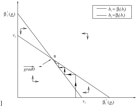
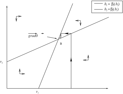
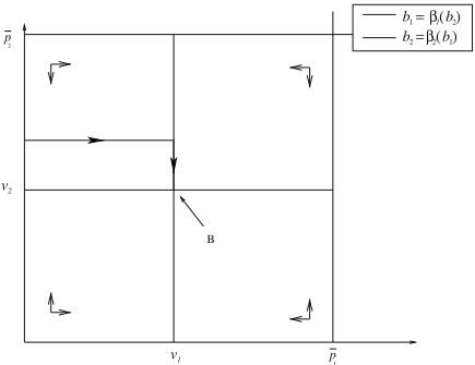
Figures 1, 2, and 3 provide a visual description of the above discussion. Each figure represents the bid domain B where N = 2 and hence we draw the two hyper-surfaces. We chose uniform probability distributions to represent the closing price distributions as a result of which the hyper-surfaces are lines. Arrows give the direction to follow to improve the expected utility in the zones delimited by the hyper-surfaces. Paths leading to local maxima are drawn as dashed lines with arrows representing the direction to follow.
Figures 1, 2, and 3 allow us to present some conclusions. For all types of item valuations, it is preferable to bid the individual valuation of an item when bidding only for this item. For substitutable items, βi is decreasing and the maximum value taken by βi is βi(pi) = vi where vi = ϑ({i}), and the bidder should always bid less than its individual valuation for each item when bidding for a bundle. On the contrary, for complementary items, βi is increasing and the minimum value taken by βi is βi(pi) = vi, and the bid for an item should always be more than the individual valuation for that item when bidding for an item bundle.
In the examples presented in these figures, we have unique optima. Given the nature of the closing price distributions, however, the N hyper-surfaces may have several intersections resulting in as many local optima. Consequently, we can only guarantee reaching a local maxima using the N-sequential MDBI process. This problem can be circumvented by restarting the improvement process, e.g., by choosing a random bid vector, when no further improvement is possible. Assuming an infinite number of restarts, this method will discover the optimal bid vector. As this is not feasible in practice, only a finite number of restarts can be considered.
We observe that for non-related items, and irrespective of the number of items, there exists a unique optimum. Indeed, in that case, βi(bi) = vi. Consequently, the N hyper-surfaces are orthogonal (see Figure 3) and therefore have a unique intersection ˆB = (v1, . . . , vN) which corresponds to B∗ . Starting from any bid vector, we will arrive at this solution using the MDBI scheme. As a result, the MDBI process will output the optimal bid vector irrespective of of initial bids when items are non-related.
4.2 Bidding Algorithm
We now describe the steps of our bid improvement algorithm in more detail. An initial bid vector B0 is chosen. Let Bt be the bid after t iterations. Bt+1 is obtained by improving sequentially bids for each of the N items in Bt, keeping the bids for other items constant. The process is stopped when ||Bt+1 - Bt|| < ε where ε is a user-chosen positive constant and || · || is any vectorial norm. To improve a bid, we need to calculate βi. Though the formula presented in Proposition 2 requires exponential computation, it is possible to approximate βi in polynomial time via price sampling. Algorithm 1
1
Figure 3: Hyper-surfaces when N = 2, closing price distributions are uniform, and items are non-related.
presents the pseudo-code to approximate βi. Algorithm 2 presents the pseudo-code for the MDBI algorithm.
Algorithm 1 Approximation of βi(B-i) by price sampling
Algorithm 2 MDBI
B ← initializeBids() // Improvement loop. repeat B′ = B for i = 1..N do end for until ||B -B′ || < εbi ← βapprox(i, B-i, F, ϑ, K) return BThe computational complexity of approximating βi(B-i), βapprox(i, B-i, F, ϑ, K), is linear given the number of samples, K. More precisely, it is equal to θ(K) additions, θ(K) valuation calculations and θ(K) price sample generations. In MDBI, each N-sequential improvement requires N approximations of βi(B-i). The number of N-sequential improvement depends on the number of iterations of the improvement loop, C(ε, N). We have (C(ε, N) ∗ N) N-sequential improvement and C(ε, N) calculations of norms. Generally, vectorial norms can be computed in linear time given the dimension of the space (N in our case). Thus, the complexity of MDBI is O(KN C(ε, N)) additions, O(KN C(ε, N)) valuation calculations and O(KN C(ε, N)) price sample generations. The value of C(ε, N) is difficult to judge a priori but experimental results presented in the next section show that C(ε, N) increases only very gradually with N and thus the computational complexity of MDBI is approximately linear. This, in particular, is a significant improvement over current schemes [Greenwald and Boyan, 2004; Stone et al., 2003] which have exponential complexity.
5 Experimental results
We ran experiments with the following objectives: to show that our algorithm performs well when probability distributions are discrete 2 , both in terms of the quality of the solution provided and the time efficiency 3 . We compare variants of our algorithms with an exhaustive search or brute force algorithm (BF) that provides optimal results at high search costs. The BF approach consists of calculating the expected profit generated by each possible bid combinations and then bidding the best combination. BF is optimal, but its complexity is exponential. We now present three variants of our MDBI algorithm that we have experimented with:
2 Our study was made assuming continuous distributions. In reallife environments, agents are likely to use discrete probability distributions.
3 Though we provide formal analysis of the complexity of our algorithm, the expression of MDBI complexity contains a function (C(ε, N)) whose value is unknown. The goal of our experiments is to see whether C(ε, N) scales minimally with N.
- RandomStart Bid Improver (RSMDBI): RSMDBI starts with a randomly chosen bid vector and does not use restarts.
- Random Start Bid Improver With Restart (RSMDBIWRn):
RSMDBIWRn starts with a randomly chosen bid vector and restarts the hill-climbing process n - 1 times and outputs the bid vector with the highest expected utility.
- Valuation Start Bid Improver (VSMDBI): VSMDBI starts with the bid Bϑ1 = (v1, . . . , vN) and does not use restarts.
5.1 Experimental settings
In the first set of experiments, we used the above-mentioned variants of the MDBI algorithm in an environment containing four single-item single-unit auctions and the focus is on evaluating their success in finding optimal solutions, as checked by the BF scheme, under different valuation functions. Subsequently we present results with larger number of items where the focus is on studying the time efficiency and scaleup properties of the algorithms. All closing prices are drawn from discrete closing price distributions. A simulation consists of one bidder with the knowledge of all closing price distributions. This bidder can place one bid in all four auctions at each iteration. At the end of each iteration, the bidder knows which items it won and the payment it has to make for those items. At the end of each simulation, the average profit of the bidder is calculated. A run of our experiment consists of four simulations, one for each of the bidders RSMDBI, RSMDBIWRn with n=5 or 10, VSMDBI, BF. For a run, bidders in each simulation share the same valuation function. We generate four kinds of valuation functions: (a) SI, where items are substitutable, (b) CI, where items are complementary, (c) NRI, where items are non-related, and (d) RVI, where valuations for bundles are random. Considering three set of items I, J, K such that J ∪ K = I and J ∩ K = ∅. Items are substitutable if ϑ(I) ≤ ϑ(J) + ϑ(K) for all such item sets. Items are complementary if ϑ(I) ≥ ϑ(J)+ϑ(K) for all such item sets. Items are non-related if ϑ(I) = ϑ(J) + ϑ(K) for all such item sets. If no one of the above conditions are satisfied for all item sets, we consider the items to have random valuation. Valuation for single-item bundle is drawn from the range [0, 100], i.e., ϑ({i}) ∈ [0, 100] ∀i ∈ I. In each run, the same auctions are repeated in each simulation, i.e., the same closing price distributions are utilized for each simulation. We have eight predefined probability distributions. Four of them produce price ranges from 10 to 90 and four of them from 60 to 140 with discrete values in increments of 10. For each range, one distribution is uniform (UP), one outputs the highest prices with higher probability (HP), one outputs the lowest prices with higher probability (LP), and one outputs price in the middle of the range with higher probability (MP).
For each run, distributions for the four auctions are chosen randomly.
5.2 Quality of solutions provided by algorithms
To compare our algorithms, we display the cumulative average profit generated by the bidders using each strategy in Table 1. Algorithms are ordered by the net utility obtained. Horizontal lines in the table groups the algorithms into blocks. Performance of algorithms in the same block are statistically indistinguishable according to the Wilcoxon test.
We highlight the following observations:
- VSMDBI performs similar to RSMDBI except for RVI valuations where performances are worse.
- With a small number of random restarts our algorithm always has performance similar to BF which is asymptotically optimal.
- RSMDBIWRn with n = 5, 10 has better performances than RSMDBI except for non-related items where performances are equal. As we have observed before, restarts are unnecessary for non-related items.
- Every algorithm is optimal when items are non-related.
Remark 1 shows that choosing Bϑ1 as a starting point is a good heuristic for some but not all cases. Remark 2 shows that with reasonable number of restarts (5 in our experiments) the optimal bid vector is always found. Since RSMDBI is, in general, not optimal (Remark 3), we can say that the bid domain has, in general, some local maxima and/or ridges. However, since few restarts permit to find optimal bids, the number of local maxima and ridges is not very high. Consequently, RSMDBIWRn with reasonably small values of n can be considered as an approximately optimal method. From Remark 4, we find that almost every algorithm is optimal for NRI. Though this result is not that significant as we know the optimal bid vector in that case, it confirms our previous analysis which claimed that the optimal bids are found by the MDBI algorithm after the first N-sequential improvement irrespective of the initial bid vector.
5.3 Time efficiency and scale up properties
To evaluate the run time of our algorithm for larger problems, we run experiments as described in the last section but by changing the number of items from 4 to 15 to evaluate the values of C(ε, N). Those experiments were similar to the previous ones except that we output the values of C(ε, N) and average them. We highlight the following observations:
- Except for NRI, the number of N-sequential improvements (C(ε, N)) increases very slowly. The largest range is [2, 4].
- The number of N-sequential improvements is always better for VSMDBI.
- C(ε, N) = 1 for VSMDBI and C(ε, N) = 2 for RSMDBI when items are non-related.
We can conclude that C(ε, N) is almost constant. Consequently, the computational complexity of our algorithms is almost linear given the number of items and hence has desirable time efficiency and scale up properties. The third remark
| Strategy | Score |
|---|---|
| RSMDBIWR10 BF | 1940.2 1909.4 |
| RSMDBIWR5 | 1907.2 |
| VSMDBI | 1859.6 |
| RSMDBI | 1856.8 |
| Strategy | Score |
|---|---|
| RSMDBI | 3748.4 |
| VSMDBI | 3731.5 |
| RSMDBIWR10 | 3725.2 |
| RSMDBIWR5 | 3724.7 |
| BF | 3658.3 |
(c) NRI
| Strategy | Score |
|---|---|
| BF | 7693.4 |
| RSMDBIWR5 | 7693.3 |
| RSMDBIWR10 | 7674.7 |
| VSMDBI | 7513.8 |
| RSMDBI | 7434.8 |
(b) CI
| Strategy | Score |
|---|---|
| RSMDBIWR10 | 6898.9 |
| BF | 6871.0 |
| RSMDBIWR5 | 6828.6 |
| RSMDBI | 6239.8 |
| VSMDBI | 5946.3 |
(d) RVI
Table 1: Profits fromMDBI variants with different valuation functions.
can be explained by the fact that VSMDBI will try to improve the initial bid B0 = Bϑ1 and will realize that there is no better bid vector. RSMDBI will improve its initial bid vector and reach the optimal one B∗ = Bϑ1 in one N-sequential improvements. Then, it behaves like VSMDBI.
In a companion paper [Candale and Sen, 2006] we show that MDBI produces equal or better solutions in much less time compared to MU and EVMU algorithms for larger number of items than discussed here. We cannot verify the optimality of those results as it was computationally prohibitive to run the BF algorithm for those larger problem sizes. The experimental results clearly demonstrate the effectiveness and scalability of the MDBI schemes.
6 Conclusions
We presented a new method for bidding in simultaneous auctions which is asymptotically optimal. We used a novel optimization based technique that improves any arbitrary bid vector. While we developed the bidding approach assuming continuous closing price probability distributions, we showed that our technique is applicable when closing prices are discrete. The MDBI algorithm performs optimally with few restarts and also scales up well with the number of items.
The MDBI algorithm produces optimal bid vectors with infinite random restarts. As this is infeasible in practice, we evaluate variants of the scheme with finite number of restarts and carefully chosen starting bid vectors. A surprising result is that good solutions can be achieved without restarts when items are substitutable, complementary, or are non-related. In general, small number of restarts can be used to approximate optimal expected utility in all cases.
A desirable property of our algorithm, in contrast to existing schemes, is its approximately linear time complexity. Experimental results show that the MDBI scheme scales up effectively with larger number of items.
We plan to study situations where a bidder can bid in both single-item and combinatorial auctions to acquire bundles. We also intend to adapt MDBI for generating bids for multiunit auctions.
Acknowledgment US National Science Foundation award IIS-0209208 partially supported this work.
@inproceedings{ijcai2007p196,
  title     = {Multi-Dimensional Bid Improvement Algorithm for Simultaneous Auctions},
  author    = {Candale, Teddy and Sen, Sandip},
  booktitle = {Proceedings of the Twentieth International Joint Conference on
               Artificial Intelligence, {IJCAI-07}},
  publisher = {International Joint Conferences on Artificial Intelligence},
  editor    = {Manuela M. Veloso},
  pages     = {1215--1219},
  year      = {2007},
  url       = {https://ijcai.org/proceedings/2007/196},
}
TY - CPAPER TI - Multi-Dimensional Bid Improvement Algorithm for Simultaneous Auctions AU - Candale, Teddy AU - Sen, Sandip T2 - Proceedings of the Twentieth International Joint Conference on Artificial Intelligence, IJCAI-07 PB - International Joint Conferences on Artificial Intelligence PY - 2007 SP - 1215 EP - 1219 UR - https://ijcai.org/proceedings/2007/196 ER -Copied
Machine-readable versions of this paper, for tools and AI agents:





