
Protein Quaternary Fold Recognition Using Conditional Graphical Models
Proceedings of the Twentieth International Joint Conference on Artificial Intelligence. Pages 937-944.
© 2007 International Joint Conferences on Artificial Intelligence
Abstract
Protein fold recognition is a crucial step in inferring biological structure and function. This paper focuses on machine learning methods for predicting quaternary structural folds, which consist of multiple protein chains that form chemical bonds among side chains to reach a structurally stable domain. The complexity associated with modeling the quaternary fold poses major theoretical and computational challenges to current machine learning methods. We propose methods to address these challenges and show how (1) domain knowledge is encoded and utilized to characterize structural properties using segmentation conditional graphical models; and (2) model complexity is handled through efficient inference algorithms. Our model follows a discriminative approach so that any informative features, such as those representative of overlapping or long-range interactions, can be used conveniently. The model is applied to predict two important quaternary folds, the triple beta-spirals and double-barrel trimers. Cross-family validation shows that our method outperforms other state-of-the art algorithms.
- [Altschul et al., 1997] SF Altschul, TL Madden, AA Schaf- fer, J Zhang, Z Zhang, W Miller, and DJ. Lipman. Gapped BLAST and PSI-blast: a new generation of protein database search programs. Nucleic Acids Res., 25(17):3389-402, 1997.
- [Andrieu et al., 2000] Christophe Andrieu, Nando de Fre- itas, and Arnaud Doucet. Reversible jump mcmc simu- lated annealing for neural networks. In Proceedings of UAI-00, 2000.
- [Bateman et al., 2004] Alex Bateman, Lachlan Coin, Richard Durbin, Robert D. Finn, Volker Hollich, Sam Griffiths-Jones, Ajay Khanna, Mhairi Marshall, Simon Moxon, Erik L. L. Sonnhammer, David J. Studholme, Corin Yeats, and Sean R. Eddy. The pfam protein families database. Nucleic Acids Research, 32:138-141, 2004.
- [Benson et al., 2004] SD Benson, JK Bamford, DH Bam- ford, and RM. Burnett. Does common architecture reveal a viral lineage spanning all three domains of life? Mol Cell., 16(5):673-85, 2004.
- [Boys and Henderson, 2001] R J Boys and D A Henderson. A comparison of reversible jump mcmc algorithms for dna sequence segmentation using hidden markov models. Comp. Sci. and Statist., 33:35-49, 2001.
- [Cheng and Baldi, 2006] Jianlin Cheng and Pierre Baldi. A machine learning information retrieval approach to protein fold recognition. Bioinformatics, 22(12):1456-63, 2006.
- [Ding and Dubchak, 2001] C.H. Ding and I. Dubchak. Multi-class protein fold recognition using support vector machines and neural networks. Bioinformatics., 17:349- 58, 2001.
- [Durbin et al., 1998] R. Durbin, S. Eddy, A. Krogh, and G. Mitchison. Biological sequence analysis: probabilistic models of proteins and nucleic acids. Cambridge Univer- sity Press, 1998.
- [Green, 1995] Peter J. Green. Reversible jump markov chain monte carlo computation and bayesian model determina- tion. Biometrika, 82:711-732, 1995.
- [Jones et al., 1992] DT Jones, WR Taylor, and JM. Thorn- ton. A new approach to protein fold recognition. Nature., 358(6381):86-9, 1992.
- [Lafferty et al., 2001] John Lafferty, Andrew McCallum, and Fernando Pereira. Conditional random fields: Proba- bilistic models for segmenting and labeling sequence data. In Proc. of ICML'01, pages 282-289, 2001.
- [Liu et al., 2005] Yan Liu, Jaime Carbonell, Peter Weigele, and Vanathi Gopalakrishnan. Segmentation conditional random fields (SCRFS): A new approach for protein fold recognition. In Proceedings of RECOMB'05, 2005.
- [Sarawagi and Cohen, 2004] Sunita Sarawagi and William W. Cohen. Semi-markov conditional ran- dom fields for information extraction. In Proc. of NIPS'2004, 2004.
- [Taskar et al., 2003] B. Taskar, C. Guestrin, and D. Koller. Max-margin markov networks. In Proc. of NIPS'03, 2003.
- [van Raaij et al., 1999] MJ van Raaij, A Mitraki, G Lavigne, and S Cusack. A triple beta-spiral in the adenovirus fibre shaft reveals a new structural motif for a fibrous protein. Nature., 401(6756):935-8, 1999.
- [Weigele et al., 2003] Peter R. Weigele, Eben Scanlon, and Jonathan King. Homotrimeric, β-stranded viral adhesins and tail proteins. J Bacteriol., 185(14):4022-30, 2003.
References were extracted automatically from the PDF and may contain errors.
Full text extracted automatically from the PDF; figures, tables and equations may differ. The PDF is the version of record.
1 Introduction
Proteins, as chains of amino acids, tend to adopt unique threedimensional structures in their native environments. These structures play key roles in determining the activities and functions of the proteins. An important issue in computationally inferring the three-dimensional structures from aminoacid sequences is protein fold recognition and alignment. Given a target protein fold 1 , the task seeks to predict whether a test protein sequence adopts the fold and if so, provides its sequence-to-topology alignment against the fold.
There are different kinds of protein folds based on their structural properties. In this paper, we focus on the most complex ones, namely quaternary structural folds, which consist of multiple protein chains that form chemical bonds among Biology Department Massachusetts Institute of Technology Cambridge, MA 02139 pweigele@mit.edu the side chains of sequence-distant residues to reach a structurally stable domain. These folds commonly exist in many proteins and contribute significantly to evolutionary stability. Some examples include enzymes, hemoglobin, ion channels as well as viral adhesive and viral capsids.
1 Protein folds are typical spatial arrangements of well-defined secondary structures which appear repeatedly in different proteins
To date, there has been significant progress in protein tertiary fold (single chain topology) recognition, ranging from sequence similarity matching [Altschul et al., 1997; Durbin et al., 1998], to threading algorithms based on physical forces [Jones et al., 1992] and tomachine learningmethods [Cheng and Baldi, 2006; Ding and Dubchak, 2001]. However, there are three major challenges in protein sequence-to-structure mapping that hinder previous work from being applied to the quaternary fold recognition: (1) many proteins adopt the same structural fold without apparent sequence similarities. This property violates the basic assumption of many machine learning algorithms that similar observations tend to share the same labels; (2) amino acids distant in sequence-order (the distance is not known a priori) or on different chains may form chemical bonds in the three-dimensional structures. Most of these bonds are essential in the stability of the structures and have to be considered for accurate prediction; (3) furthermore, previous methods for predicting folds with single chains are not directly applicable because the complexity is greatly increased both biologically and computationally, when moving to quaternary multi-chain structures.
From a machine learning perspective, protein fold recognition falls in the general problem of predicting structured outputs, which learns a mapping between input variables and structured, interdependent output variables. Conditional graphical models, such as conditional random fields (CRF) [Lafferty et al., 2001], max-marginMarkov networks [Taskar et al., 2003], and semi-Markov CRF [Sarawagi and Cohen, 2004], have demonstrated successes in multiple applications. To address the challenges in protein fold recognition, we develop a new segmentation conditional graphical model. As an extension of the CRF model, it defines the hidden nodes as labels assigned to segments (subsequences corresponding to one secondary structure element) rather than to individual amino acid, then connects two nodes with edges to hypothesize chemical bonds. The conditional probability of the hidden variables (i.e. the segmentation of each structure element) given the observed sequence is defined as an exponential form of the features. In addition, efficient approximation algorithms are examined to find optimal or near-optimal solutions. Compared with previous work in CRF, our model is novel in capturing the long-range dependencies of different subunits within one chain and between chains.
The major advantages of our approach for protein fold recognition include: (1) the ability to encode the output structures (both inter-chain and intra-chain chemical bonding) using the graph; (2) dependencies between segments can be non-Markovian so that the chemical-bonding between distant amino acids can be captured; (3) it permits the convenient use of any features that measure the property of segments the biologists have identified.
The remainder of the paper is organized as follows. Section 2 introduces the basic concepts of protein structures and fold recognition; section 3 describes the details of our model, followed by a discussion of efficient inference algorithms for training and testing. In section 5, we give two examples of the quaternary folds and show our successful experimental results. The paper concludes with suggestions for future work.
2 Protein Structure Basics and Fold Recognition
To study protein structures, biologists have defined four conceptual hierarchies based on current understanding: the primary structure simply refers to the linear chain of amino acids; the secondary structure can be thought of as the local conformation of protein chains, or intuitively as building blocks for its global 3D structures. There are three types of standard secondary structures in nature, i.e. α-helix, a rodshape peptide chain coiled to form a helix structure, β-sheets, two or more peptide strands aligned in the same direction (parallel β-sheet) or opposite direction (antiparallel β-sheet) and stabilized by hydrogen bonds. These two types of secondary structures are connected by the remaining irregular regions, referred to as coil. The tertiary structure is the global three-dimensional structures of a single protein chain. Sometimes multiple chains are associated with each other and form a unified structure, i.e. the quaternary structures.
Protein folds are identifiable spatial arrangements of secondary structures. It is observed that there exist only a limited number of topologically distinct folds in nature (around 1,000) although we have discovered millions of protein sequences. As a result, proteins with the same fold often do not demonstrate sequence similarities, which might reveal important information about structural or functional conservation due to common ancestors. An example is the triple βspiral fold, a processive homotrimer which serves as a fibrous connector from the main virus capsid to a C-terminal knob that binds to host cell-surface receptor proteins. The fold has been identified to commonly exist in adenovirus (a DNA virus which infects both humans and animals), reovirus (an RNA virus which infects human) and bacteriophage PRD1 (a DNA virus infecting bacteria), however, the similarity between these protein sequences are very low (below 25% similarity). Identifying more examples of the triple β-spiral fold will not only help the biologists to establish that it is a common fold in nature, but also reveal important evolutionary relationships between the viral proteins.
The example above motivates the task of accurate protein fold recognition and alignment prediction. The problem setting is as follows: given a target protein fold, as well as a set of N training sequences x(1) , x(2) , . . . , x(N) including both positive and negative examples with structural annotation, i.e. 3-D coordinates of each atom in the proteins, predict whether a new test sequence xtest (without structural annotation) adopts the fold or not, and if yes, identify its specific location in the sequence.
3 Representation of Domain Knowledge
It can be seen that the fold recognition task is a typical segmentation and labeling problem except that we need to address the following questions to represent the domain knowledge: how to (1) represent the states and (2) capture the structural information within the observed sequences?
The chemical bonding physically exists at the atomic level on the side-chains of amino acids, however, the structural topology and interaction maps are conserved only at the secondary structure level due to the many possible insertions or deletions in the protein sequence. Therefore it is natural for the state labels to be assigned to segments (subsequences corresponding to one secondary structure element) rather than to individual amino acids, and then connect nodes with edges indicating their dependencies in three-dimensional structures. Next, we define the formal representation of the structure information in the protein fold and discuss how to incorporate domain-knowledge features to help the prediction.
3.1 Protein Structure Graph (PSG)
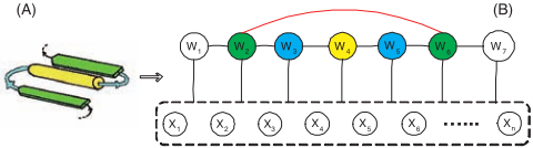
An undirected graph G =< V, E >, called protein structure graph (PSG), can be defined for the target protein fold, where V = U ⋃{I}, U is the set of nodes corresponding to the secondary structure elements within the fold and I is the node to represent the elements outside the fold. E is the set of edges between neighboring elements in sequence order (i.e. the polypeptide bonding) or edges indicating longrange dependencies between elements in three-dimensional structures (i.e. chemical bonding, such as hydrogen bonds or disulfide bonds). Figure 1 shows an example of the simple βα-β motif. Notice that there is a clear distinction between the edges colored in red and those in black in terms of probabilistic semantics: similar to a chain-structured CRF, the black edges indicate state transitions between adjacent nodes; the red edges are used to model long-range interactions, which are unique to the protein structure graph. The PSG for a quaternary fold can be derived similarly: first construct a PSG for each component protein or a component monomeric PSG for homo-multimers, and then add edges between the nodes from different chains if there are chemical bonds, forming a more complex but similarly-structured quaternary PSG.
Given the definition of the protein structure graph, our next question is how to automatically build the graph for a particular fold. The answer depends on the type of protein folds of concern and how much knowledge we can bring to bear. For folds that biologists have studied over the years and accumulated some basic knowledge of their properties (for example β-α-β motif or β-helix), the topology of this graph can be constructed easily by communicating with the experts. If it is a fold whose structure is totally unknown to biologists, we can follow a general procedure with the following steps: first, construct a multiple structure alignment of all the positive proteins (among themselves); second, segment the alignment into disjoint parts based on the secondary structures of the majority proteins; third, draw a graph with nodes denoting the resulting secondary structure elements and then add edges between neighboring nodes. Finally, add the longrange interaction edge between two nodes if the average distance between all the involved residues is below the threshold required for side-chain hydrogen-bonding. We skip the details of the latter case as it is a separate line of research and assume that we are given a reasonably good graph over which we perform our learning, since this is the focus of the paper.
3.2 Segmentation Conditional Graphical Models (SCGM)
Given a structure graph G defined on one chain and a protein sequence x = x1x2 . . . xN, we can have a possible segmentation label of the sequence, i.e. y = {M,w}, where M is the number of segments and wj = {sj, pj, qj}, in which sj, pj, and dj are the state, starting position and ending position of the j th segment. Following the idea of CRF, the conditional probability of a segmentation y given the observation x is defined as follows:
where Z0 is the normalization constant.
More generally, given a quaternary structure graph G with C chains, i.e. {xi|i = 1 . . .C}, we have a segmentation initiation of each chain yi = (Mi,wi) defined by the protein structure graph, where Mi is the number of segments in the ith chain, and wi,j = (si,j, pi,j, qi,j), si,j, pi,j and qi,j are the state, starting position and ending position of the j th segment. Following the same definition as above, we decompose the potential function over the cliques as a product of unary and pairwise potentials:
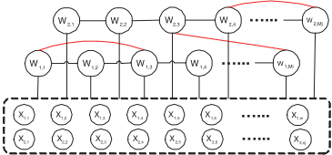
where fk and gk are node-features and pair features respectively, θ1,k and θ2,k are the corresponding weights, and Z is the normalizer over possible segmentation configurations of all the sequences jointly (see Figure 2 for its graphical model representation). Notice that joint inference is required since the quaternary fold is stabilized by the chemical bonding between all component proteins and that is the key computational challenge.
3.3 Feature Extraction
The SCGM model provides an expressive framework to handle the structural properties for protein fold recognition. However, the choice of feature functions fk and gk play a key role in accurate predictions. Following the feature definition in the CRF model, we factor the features as follows: fk(xi,wi,j) = f ′k (xi, pi,j, qi,j) if si,j = s and qi,j - pi,j ∈ length range(s), 0 otherwise. gk(xa, xb, wa,u, wb,v) = g′k (xa, xb, pa,u, qa,u, pb,v, qb,v) if sa,u = s, sb,v = s′ , qa,u - pa,v ∈ length range (s), and qb,v - pb,v ∈ length range (s′ ), 0 otherwise.
Next we discuss how to define the segment-based features f ′k and g′k . The node feature f ′k covers the properties of an individual segment, for example, "whether a specific motif appears in the subsequence", "averaged hydrophobicity", or "the length of the segment". The pairwise feature g′k captures the dependencies between segments whose corresponding subsequences form chemical bonds in the 3-D structures. For example, previous work in structural biology suggests different propensities to form the bonds between the amino acids pairs. Therefore the pairwise features could be the propensity scores of the two subsequences to form hydrogen bonds. Notice that the feature definitions can be quite general, not limited to the examples above. The discriminative setting of the model enables us to use any kinds of informative features without additional costs.
4 Efficient Inference
To find the best conformation of test sequences, we need to consider the labels of all the protein chains jointly since every chain contributes to the stability of the structures. Given the enormous search spaces in quaternary folds, we need to find efficient inference and learning algorithms.
4.1 Training Phase
The feature weights {θ1,k} and {θ2,k} are the model parameters. In the training phase, we estimate their values by maximizing the regularized conditional probability of the training data, i.e
There is no closed form solution to the equation above, therefore we use the iterative searching algorithm L-BFGS (a limited-memory quasi-Newton code for large-scale unconstrained optimization). Taking the first derivative of the log likelihood L(θ1, θ2), we have
Since PSGs may be complex graphs with loops and multiple chains (with an average degree of 3-4 for each node), we explored efficient approximation methods to estimate the feature expectation. There are three major approximation approaches in graphical models: sampling, variational methods and loopy belief propagation. Sampling techniques have been widely used in the statistics community, however, there is a problem if we use the naive Gibbs sampling. Notice that in each sampling iteration the dimension of hidden variables yi varies in cases where the number of segments of Mi is also a variable (e.g. unknown number of structural repeats in the folds). Reversible jump Markov chain Monte Carlo (reversible jump MCMC) algorithms have been proposed to solve the problem and demonstrated success in various applications, such as mixture models [Green, 1995] and hidden Markov model for DNA sequence segmentation [Boys and Henderson, 2001].
Reversible Jump Markov chain Monte Carlo
Given a segmentation yi = (Mi,wi), our goal is propose a new move y∗ i . To satisfy the detailed balance defined by the MCMC algorithm, auxiliary random variables v and v∗ have to be introduced. The definitions for v and v∗ should guarantee the dimension-matching requirement, i.e. D(yi) + D(v) = D(y∗ i ) + D(v′ ) and there is a one-to-one mapping from (yi, v) to (y∗ i , v′ ), namely a function Ψ so that Ψ(yi, v) = (y∗ i , v′ ) and Ψ-1 (y∗ i , v′ ) = (yi, v). The acceptance rate for the proposed transition from yi to y∗ i is
min{1, posterior ratio × proposal ratio × Jacobian}
where the last term is the determinant of the Jacobian matrix.
To construct a Markov chain on the sequence of segmentations, we define four types of Metropolis operators:
(1) State Transition: given a segmentation yi = (Mi,wi), select a segment j uniformly from [1,M], and a state value s′ uniformly from state set S. Set y∗ i = yi except that s∗i,j = s′ . (2) Position Switching: given a segmentation yi = (Mi, wi), select the segment j uniformly from [1,M] and a position assignment d′ ∼ U[di,j-1 + 1, di,j+1 - 1]. Set y∗ i = yi except that d∗i,j = d′ .
(3) Segment Split: given a segmentation yi = (Mi,wi), propose y∗ i = (M ∗ i ,wi ∗ ) with M ∗ i = Mi + 1 segments by splitting the j th segment, where j is randomly sampled from U[1,M]. Set w∗ i,k = wi,k for k = 1, . . . , j - 1, and w∗ i,k+1 = wi,k for k = j + 1, . . . ,Mi. Sample d∗j+1 from U [dj + 1, dj+1 - 1]. With probability 12 , we set sj∗ = sj and sj+1∗ = snew with snew sampled from S and with probability 12 do the reverse.
(4) Segment Merge: given a segmentation yi = (Mi,wi), propose M ⋆ i = Mi-1 by merging the j th segment and j+1th segment, where j is sampled uniformly from [1,M - 1]. Set w∗ i,k = wi,k for k = 1, . . . , j - 1, and w∗ i,k-1 = wi,k for k = j + 1, . . . ,Mi..
In general, many protein folds have regular arrangements of the secondary structure elements so that the state transitions are deterministic or almost deterministic. Therefore the operator for state transition can be removed and segment split or merge can be greatly simplified. There might be cases where the inter-chain or intra-chain interactions are also stochastic. Then two additional operators are necessary, including segment join (adding an interaction edge in the protein structure graph) and segment separate (deleting an interaction edge in the graph). The details are similar to state transition, and we omit the discussion due to limited space.
4.2 Testing Phase
Given a test example with multiple chains {x1, . . . , xC}, we need to search the segmentation that yields the highest conditional likelihood. Similar to the training phase, it is an optimization problem involving search in multi-dimensional space. Since it is computationally prohibitive to search over all possible solutions using traditional optimization methods, simulated annealing with reversible jump MCMC is used. It has been shown theoretically and empirically to converge onto the global optimum [Andrieu et al., 2000]. ALGORITHM-1 shows the detailed description of reversible jump MCMC simulated annealing. β is a parameter to control the temperature reduction rate, which is set to 0.5 in our experiments for rapid convergence.
5 Experiments
To demonstrate the effectiveness of different recognition models, we choose two protein folds as examples, including the triple β-spiral [van Raaij et al., 1999], a virus fiber, and the double-barrel trimer [Benson et al., 2004], which is a building block for the virus capsid hexons. We choose these two folds specifically because they are both involved in important biological functions and shared by viruses from different species, which might reveal important evolution relationships in the viral proteins. Moreover, TBS should fit our Algorithm-1: Reversible Jump MCMC Simulated Annealing Input: initial value of y0, Output: optimized assignment of y
- Set ˆy = y0.
- For t ← 1 to ∞ do :
- T ← βt. If T = 0 return ˆy
- Sample a value from ynew using the reversible jump MCMC algorithm as described in Section 4.1. ∇E = P (ynew - P (ˆy)
)
- if ∇E > 0, then set ˆy = ynew ; otherwise set ˆy = ynew with probability exp(∇E/T )
- Return ˆy
predictive framework well because of the structure repeats while DBT could be extremely challenging due to the lack of structural regularity. Both folds have complex structures with few positive examples in structurally-resolved proteins. Notice that our model may be used for any protein folds, however their advantages are most evident in predicting these complex and challenging protein folds.
5.1 Protein Structure Graph of Target Fold
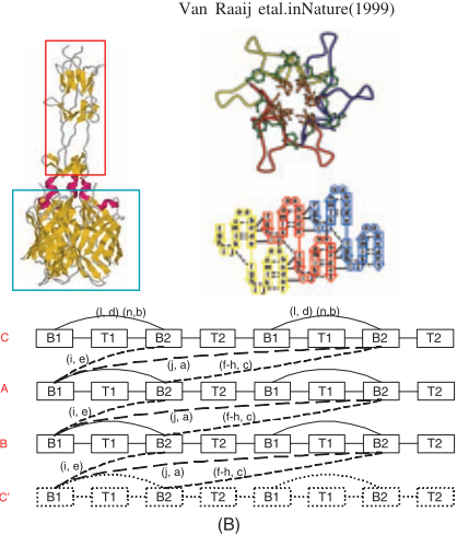
Triple β-spiral fold (TBS) is a processive homotrimer consisting of three identical interacting protein chains (see Figure 3). It provides the structural stability for the adhesion protein to initiate a viral attack upon the target cell wall. Up to now there are three proteins of this fold with resolved structures. However, its common existence in viruses of different species reveals important evolutionary relationships. It also indicates that TBS might be a common fold in nature although very few examples have been identified so far.
To provide a better prediction model, we notice the following structural characteristics in TBS: it consists of three identical protein chains with a varied number of repeated structural subunits. Each subunit is composed of: (1) a β-strand that runs parallel to the fiber axis; (2) a long solvent-exposed loop of variable lengths; (3) a second β-strand that forms antiparallel β-sheets with the first one, and slightly skewed to the fiber axis; (4) successive structural elements along the same chain are connected together by tight β-turns [Weigele et al., 2003]. Among these four components, the two βstrands are quite conserved in sequences and van Raaij et al. characterize them by labeling each position using character 'a' to 'o' [van Raaij et al., 1999]. Specifically, i-o for the first strand and a-h for the second strand (see Figure 3-(Topright)). Based on the discussion above, we define the PSG for the TBS fold in Figure 3. There are 5 states altogether, i.e. B1, T1, B2 and T2, which correspond to the four components of each repeated structural subunits respectively, and the null state I, which refers to the non-triple β-spiral region. We fix the length of B1 and B2 as 7 and 8 respectively due to their sequence conservation; in addition, we set the length of T1 and T2 in [0, 15] and [0, 8] individually since longer insertions will bring instability to the structures (this is an example of prior biological knowledge constraining the model space). The pairs of interacting residues are marked on the edges, which are used to define the pairwise features.
Double-barrel trimer (DBT) is a protein fold found in the coat proteins from several kinds of viruses. It has been suggested that the occurrence of DBT is common to all icosahedral dsDNA viruses with large facets, irrespective of its host [Benson et al., 2004]. However, it is not straightforward to uncover the structural conservation through sequences homology since there are only four positive proteins and the sequence similarity is low.
The DBT fold consists of two eight-stranded jelly rolls, or β-barrels (see Figure 4). The eight component β-strands are labeled as B, C, D, E, F, G, H and I respectively. Some general descriptive observations include: (1) the lengths of the eight β-strands vary, ranging from 4 to 16 residues, although the layout of the strands is fixed. The loops (insertions) between the strands are in general short (4 - 10 residues), however, there are some exceptions, for example the long insertions between the F and G strand (20 - 202 residues); further long loops between D-E strand (9 - 250 residues); and the short βturn between E and F. (2) The chemical bonds that stabilize the trimers are located between the FG loops. Unfortunately, the specific location and bonding type remain unclear. We denote the FG loop in the first double-barrel trimer as FG1, and that in the second one as FG2. Based on the discussion above, we define the PSG of the double-barrel trimer as shown in
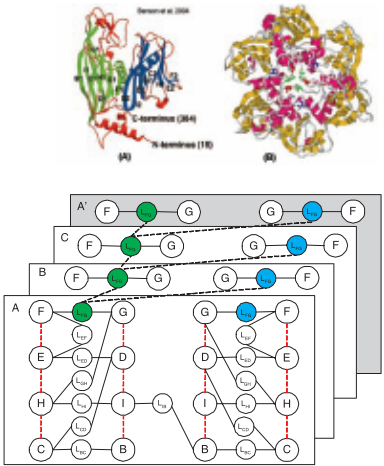
Figure 4. There are 17 states in the graph altogether, i.e. B, C, D, E, F, G, H, I as the eight β-strands in the β-barrels, lBC, lCD, lDE, lEF , lFG, lGH, lHI, lIB as the loops between the β-strands. The length of the β-strands are in the range of [3, 16]. The length range of the loops lBC, lCD, and lEF is [4, 10]; that of lDE and lFG is [10, 250]; that of lGH, lHI , lIB is [1, 30].
5.2 Experiment Results
In the experiments, we test our hypothesis by examining whether our model can score the known positive examples higher than the negative ones by using the positive sequences from different protein families in the training set. Following the setup described in [Liu et al., 2005], we construct a PDBminus dataset as negative examples (2810 proteins in total), which consists of all non-homologous proteins with known structures and confirmed not having the TBS (or DBT) fold. A leave-family-out cross-validation was performed (withholding all the positive proteins from the same family) 2 . Similarly, the PDB-minus set was also randomly partitioned into three subsets, one of which is placed in the test set while the rest serve as the negative training examples. Since negative data dominate the training set, we subsample only 10 negative sequences most similar to the positive ones. The node features include template matching and HMM profile score for B1 and B2 motifs (for TBS fold), averaged secondary structure prediction score, hydrophobicity, solvent accessibility and ionizable scores. The pairwise features include side-chain alignment score as well as parallel/anti-parallel βsheet alignment score. We compare our results with standard sequence similarity-based algorithm PSI-BLAST [Altschul et al., 1997], profile hidden-Markov model methods, Pfam [Bateman et al., 2004] and HMMER [Durbin et al., 1998] with structural alignment, as well as free-energy based algorithm Threader [Jones et al., 1992]. For our model, the number of iterations in simulated annealing is set to 500. It may not provide the globally optimal solutions, but the suboptimal ones we get seem to be very reasonable as shown below. The rank is sorted based on the log ratio of the probability of the best segmentation to that of degrading into one segment with null state.
2 Cross-family prediction is both more useful and more challenging than within family structure prediction since the latter can rely on sequence homology while the former typically cannot.
| SCOP family | Pfam | HMMER | Threader | SCGM |
| Adenovirus | 11 | 7 | 26 | 1 |
|---|---|---|---|---|
| Reovirus | 1 | 2 | 242 | 1 |
| PRD1 | 7 | 194 | 928 | 1 |
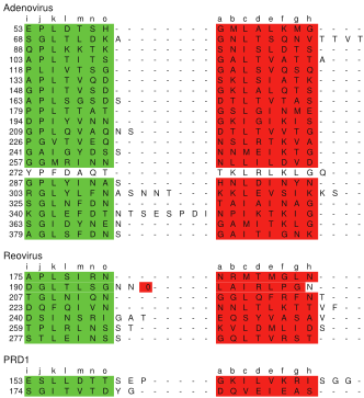
We can see all the methods except the SCGM model perform poorly for predicting the TBS fold (Table 1). With PSIBLAST, we can only get hits for the reovirus when searching against adenovirus, and vice versa. Neither can be found when we use the PRD1 as the query. The task of identifying the TBS fold is very difficult since it involves complex structures, yet there are only three positive examples. However, our methods not only can score all the known triple β-spirals higher than the negative sequences, but also is able to recover most of the repeats from the segmentation (Figure 5). The next step is to predict the presence of the TBS fold on proteins with unresolved structures, leading to targeted crystallography experiments for validation.
| SCOP family | Seq-H | Struct-H | Threader | SCGM |
|---|---|---|---|---|
| Adenovirus | 12 | 14 | > 385 | 87 |
| PRD1 | 84 | 107 | 323 | 8 |
| PBCV | 92 | 8 | 321 | 3 |
| STIV | 218 | 70 | 93 | 2 |
From Table 2, we can see that it is an extremely difficult task to predict the DBT fold. Our method is able to give higher ranks for 3 of the 4 known DBT proteins, although we are unable to reach a clear separation between the DBT proteins and the rest. The results are within our expectation because the lack of signal features and unclear understanding about the inter-chain interactions makes the prediction significantly harder. We believe more improvement can be achieved by combining the results from multiple algorithms.
6 Conclusion
In this paper, we presented a new and effective learning model, the segmentation conditional graphical model, for protein quaternary fold recognition. A protein structure graph is defined to capture the structural properties. Following a discriminative approach, our model permits the use of any types of features, such as overlapping or long-range interaction features. Due to the complexity of the graph, reversible jump MCMC is used for inference and optimization. Our model is applied to predict the triple β-spiral and doublebarrel trimer fold with promising results. Furthermore, since the long-range dependencies are common in many other applications, such as machine translation, we anticipate that our approach can be productively extended for other tasks.
Acknowledgments
This material is based upon work supported by the National Science Foundation under Grant No. 0225656. We thank anonymous reviewers for their valuable suggestions.
@inproceedings{ijcai2007p151,
  title     = {Protein Quaternary Fold Recognition Using Conditional Graphical Models},
  author    = {Liu, Yan and Carbonell, Jaime G. and Gopalakrishnan, Vanathi and Weigele, Peter},
  booktitle = {Proceedings of the Twentieth International Joint Conference on
               Artificial Intelligence, {IJCAI-07}},
  publisher = {International Joint Conferences on Artificial Intelligence},
  editor    = {Manuela M. Veloso},
  pages     = {937--944},
  year      = {2007},
  url       = {https://ijcai.org/proceedings/2007/151},
}
TY - CPAPER TI - Protein Quaternary Fold Recognition Using Conditional Graphical Models AU - Liu, Yan AU - Carbonell, Jaime G. AU - Gopalakrishnan, Vanathi AU - Weigele, Peter T2 - Proceedings of the Twentieth International Joint Conference on Artificial Intelligence, IJCAI-07 PB - International Joint Conferences on Artificial Intelligence PY - 2007 SP - 937 EP - 944 UR - https://ijcai.org/proceedings/2007/151 ER -Copied
Machine-readable versions of this paper, for tools and AI agents:





