
Distance Constraints in Constraint Satisfaction
Proceedings of the Twentieth International Joint Conference on Artificial Intelligence. Pages 106-110.
© 2007 International Joint Conferences on Artificial Intelligence
Abstract
Users can often naturally express their preferences in terms of ideal or non-ideal solutions. We show how to reason about logical combinations of distance constraints on ideals and non-ideals using a novel global constraint. We evaluate our approach on both randomly generated and real-world configuration problem instances.
- [Angelsmark and Thapper, 2004] O. Angelsmark and J. Thapper. New algorithms for the maximum Hamming distance problem. In Proceedings of CSCLP, 2004.
- [Artiouchine and Baptiste, 2005] K. Artiouchine and P. Baptiste. Inter-distance constraint: An extension of the all-different con- straint for scheduling equal length jobs. In CP, pp.62-76, 2005.
- [Bailleux and Marquis, 1999] O. Bailleux and P. Marquis. DISTANCE-SAT: Complexity and algorithms. In AAAI/IAAI, pp.642-647, 1999.
- [Bistarelli et al., 1997] S. Bistarelli, U. Montanari, and F. Rossi. Semiring-based constraint satisfaction and optimization. J. ACM, 44(2):201-236, 1997.
- [Boutilier et al., 2004] C. Boutilier, R.I. Brafman, C. Domshlak, H.H. Hoos, and D. Poole. Cp-nets: A tool for representing and reasoning with conditional ceteris paribus preference statements. JAIR, 21:135-191, 2004.
- [Hebrard et al., 2005] E. Hebrard, B. Hnich, B. O'Sullivan, and T. Walsh. Finding diverse and similar solutions in constraint pro- gramming. In AAAI, pp.372-377, 2005.
- [Régin and Rueher, 2000] J.-C. Régin and M. Rueher. A global constraint combining a sum constraint and difference constraints. In CP, pp.384-395, 2000.
- [Rossi and Sperduti, 2004] F. Rossi and A. Sperduti. Acquiring both constraint and solution preferences in interactive constraint systems. Constraints, 9(4):311-332, 2004.
References were extracted automatically from the PDF and may contain errors.
Full text extracted automatically from the PDF; figures, tables and equations may differ. The PDF is the version of record.
1 Introduction
In many application domains users specify their desires in terms of assignments to (a subset of) problem variables. For example, when planning a vacation, a user might have an ideal holiday in mind. This ideal holiday might, however, be infeasible. Consider as another example purchasing a car. The user might like two models on display (say Volvo and Jaguar). Moreover, she does not like at all a third model (say Lada). As a result, she might want to sample models similar to Volvo and Jaguar whilst different from Lada. She might therefore specify "I would like something either like the Volvo or the Jaguar, but not the Lada". This type of query is difficult to tackle using usual constraint-based preferences since it is not articulated in terms of variables and/or constraints but rather (partial) solutions. Many formalisms for representing preferences in constraint satisfaction assign preferences to individual constraints [Bistarelli et al., 1997]. Others, such as CP-Nets [Boutilier et al., 2004], specify preferences at a variable level. However, users often like to describe their preferences at a solution level [Rossi and Sperduti, 2004].
In this paper we present an algebra for complex expressions of distance constraints. We describe a novel soft global constraint for propagating constraints of distance, characterise the conditions under which we can propagate it tractably, and report encouraging results on real-world and randomly generated instances.
2 Preliminaries
A constraint satisfaction problem (CSP) is a triple P ˆ= 〈X,D, C〉 where X is a finite set of variables X ˆ= {x1, . . . , xn}, D is a set of finite domains D ˆ= {D(x1), . . . ,D(xn)} where the domain D(xi) is the finite set of values that variable xi can take, and a set of constraints Toby Walsh NICTA and UNSW Sydney, Australia tw@cse.unsw.edu.au C ˆ= {c1, . . . , cm}. Each constraint ci is defined by an ordered set var(ci) of variables and a set sol(ci) of allowed combinations of values. An assignment of values to the variables in var(ci) satisfies ci if it belongs to sol(ci). A feasible solution is an assignment to each variable of a value from its domain such that every constraint in C is satisfied. In addition to the CSP, we assume that we have some symmetric, reflexive, total and polynomially bounded distance function, δ, between (partial) instantiations of the variables, i.e. an assignment of values to some subset of X. To make reasoning easier, we assume that distance is decomposable into a sum of distances between the assignments to individual variables. For example, we might have the Hamming distance given by ∑i (X[i] ̸= Y [i]), or the generalised Manhattan distance given by ∑i |X[i] - Y [i]|.
3 Problems of Distance
We suppose the user expresses her preferences in terms of ideal or non-ideal (partial) solutions. Partiality is important so we can ignore irrelevant attributes. For example, we might not care whether our ideal car has run-flat tires or not. The fundamental decision problems underlying our approach ensure that a solution is at a given distance to (resp. from) an ideal (resp. non-ideal) solution.
dCLOSE (resp. dDISTANT)
Instance. A CSP, P, a symmetric, reflexive, total and polynomially bounded distance function δ, and p, a partial instantiation of the variables of P.
Question. Does there exist a solution s ∈ sol(P) such that δ(p, s) < d (resp. δ(p, s) ≥ d).
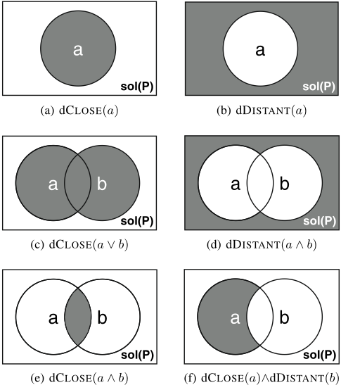
dCLOSE and dDISTANT are NP-complete in general, since they can be used to decide the CSP, P . If the distance d is not fixed, dCLOSE and dDISTANT are not necessarily polynomial even if the underlying CSP is itself polynomial [Bailleux and Marquis, 1999]. However, one can identify tractable restrictions of these problems if d is fixed and the underlying CSP is polynomial [Bailleux and Marquis, 1999]. We can specify more complex problems of distance by combining primitive distance constraints using negation, conjunction and disjunction; some examples are shown in Figure 1. The laws of our basic algebra for constructing constraint expressions are as follows (we slightly abuse the notation used to define the decision problems, without consequence) where a and b are ideal and non-ideal (partial) assignments to the variables:
dDISTANT(a) ↔ ¬dCLOSE(a) dDISTANT(a ∨ b) ↔ dDISTANT(a) ∨ dDISTANT(b) ↔ ¬dCLOSE(a ∧ b) dDISTANT(a ∧ b) ↔ dDISTANT(a) ∧ dDISTANT(b) ↔ ¬dCLOSE(a ∨ b)More complex expressions are also possible. For example, we can construct expressions using implies, iff, xor, or ifthen. Such connectives can, however, be constructed using the standard Boolean identities.
4 Optimisation problems
Rather than specify the precise distance from the ideals and non-ideals to the solution it may be more useful to minimise (maximise) the distance to an ideal (resp. a non-ideal).
CLOSE (resp. DISTANT)
Instance. A CSP, P, a distance function δ, and a partial solution p.
Question. Find a solution s ∈ sol(P) such that for all s′ ∈ sol(P) - {s}, δ(p, s) ≤ δ(p, s′ ) (resp. δ(p, s) ≥ δ(p, s′ )).
These optimisation problems are closely related to MOSTCLOSE and MOSTDISTANT defined in [Hebrard et al., 2005]. Like these problems, CLOSE and DISTANT are FPNP[log n] - complete. However, there are some differences. First, MOSTCLOSE finds the feasible solution nearest to a given subset of solutions. By comparison, CLOSE finds the feasible solution nearest to just one solution. We will soon extend CLOSE to nearness to combinations of solutions. Second, the ideal solution that CLOSE is trying to get near to might not be feasible whereas in MOSTCLOSE it is. Third, if the ideal solution is feasible then CLOSE will return it whilst MOSTCLOSE will find the next nearest feasible solution.
We can again consider logical combinations of ideals and non-ideals. For example, we might want to minimise the distance to one ideal or maximise the distance from a non-ideal. Distances can be combined in a number of ways. For example, if we want to minimise the distance to ideals a and b, we minimise the maximum distance to either. Similarly, if we want to minimise the distance to ideals a or b, we minimise the minimum distance to either. This gives us a new global objective, F, as shown in Table 1.
| Constraint | Objective function |
|---|---|
| CLOSE(a ∨ b) CLOSE(a ∧ b) | F =min(δ(s, a), δ(s, b)) F =max(δ(s, a), δ(s, b)) |
Other combinators like + and min are also possible. We also permit the distance function to depend on the ideal or non-ideal. For example, we might want distance from ideal c to count twice as much as distance from d. In this case, CLOSE(c ∨ d) gives the objective function F = min(2δ(s, c), δ(s, d)). To make combinations uniform, we convert maximising the distance, δ, from a non-ideal a into minimising a new distance, m - δ, to a where m is the maximum possible distance returned by δ. In this way, we get a single objective F which we need to minimise. Finally, we consider compiling out an objective function for a more complex logical combination of distance constraints.
Example 1 (Conjunction) We consider again the example of the choice of car configuration within a large catalogue used in Section 1. A customer is interested in two models (Volvo and Jaguar), whilst disliking a third model (Lada). The query CLOSE(Volvo), CLOSE(Jaguar), DISTANT(Lada) implements this wish. This expression means that we seek a solution s that is simultaneously as similar as possible to Volvo and Jaguar and as different as possible from Lada. It can be reformulated as the following logical expression:
(CLOSE(Volvo) ∧ CLOSE(Jaguar) ∧ DISTANT(Lada))
which gives the following objective function, F, substituting max for logical conjunction and converting maximising distance to minimising the distance complement:
5 Propagation and Complexity
We consider how to propagate such distance constraints. We observed in [Hebrard et al., 2005] that the problems MOSTCLOSE and MOSTDISTANT can be solved using symmetrically equivalent algorithms. Similarly, the problems studied here are symmetric, therefore we focus on minimising the distance (similarity) rather than maximising it (diversity). Thus, we introduce a soft global constraints SIMILAR⊗. The n-ary operator ⊗ ∈ {min,max} is used to aggregate distances to individual ideals:
The operator min handles disjunctions of distance constraints whilst max handles conjunctions. The constraint ensures that the distance to a set of ideals V = {v1, . . . , vk} is at most N. Notice that we assume that the distance between two vectors is equal to the sum of the distances on all coordinates.
We showed that enforcing generalised arc consistency (GAC) on this constraint is NP-hard for ⊗ = max [Hebrard et al., 2005]. However, enforcing GAC is tractable when the number of ideals is bounded. On the other hand, for ⊗ = min, GAC can be enforced in polynomial time for any number of ideals. Table 2 summarises the complexity of enforcing GAC on the SIMILAR⊗ constraint. We now prove the results given in this table.
Disjunction (SIMILARmin). Propagating the SIMILAR⊗ constraint for a single ideal can be done in polynomial time. Indeed, it is equivalent to the problem dCLOSE on a network involving only domain constraints. Algorithm 1 implements a linear (O(nd)) algorithm for filtering SIMILAR with respect to a single ideal (the value of ⊗ is undefined in this case).
Algorithm 1: Prune a distance constraint, single ideal. Data: X1, . . . , Xn, N, v, δ Result: GAC closure of SIMILAR([X1, . . . , Xn], N, v, δ) LB ← 0; foreach Xi do 1 lb[i] ←min(δ(v[i], j), ∀j ∈ D(Xi)); LB ← LB + lb[i] min(N) ← max(min(N), LB); 2 foreach Xi do 3 foreach j ∈ D(Xi) do if min(N) + δ(v[i], j) - lb[i] > max(N) then D(Xi) ← D(Xi) \ {j};The notation min(N) stands for the minimal value in the domain of N. Algorithm 1 first computes the smallest distance to the ideal v in loop 1. Then the domain of N and of X1, . . . ,Xn are pruned in line 2 and loop 3. For disjunctive combinations, we compute the values that are inconsistent for each distance constraint using Algorithm 1, and prune those values in the intersection. Using constructive disjunction, we achieve GAC in O(ndk) time.
| SIMILARmin | SIMILARmax | |
|---|---|---|
| k ∈ O(1) | O(ndk) | O(d2nk+2 ) |
| k ∈ O(p(n)) | O(ndk) | NP-hard |
Conjunction (SIMILARmax). Conjunctive combinations of distance constraints are more problematic. Consider the conjunctive Hamming distance constraint:
Deciding the satisfiability of this formula is NP-hard. Hence, enforcing GAC on SIMILARmax with respect to an arbitrary number of ideals is NP-hard [Hebrard et al., 2005]. However, we shall investigate filtering methods stronger than a straightforward decomposition into distance constraints with respect to a single ideal. We shall see in the next section that even though a distance constraint to a single ideal is easy to propagate and the conjunction of such constraints can naturally be processed as individual constraints in a network, stronger filtering can be obtained by considering the whole conjunction.
Algorithm 2: Lower bound on N.
Data: X1, . . . ,Xn,N, V = {v1, . . . , vk}, {δ1, . . . , δk} Result: A lower bound on N Q ← [0, 0, . . . , 0]; foreach Xi do Q′ ← ∅; foreach j ∈ D(Xi) do foreach M ∈ Q do M ′ ← M; foreach vl ∈ V do M ′ [l] ← M ′ [l] + δl(j, vl[i]); Q′ ←Q′ ∪M ′ ; Q ← Q′ ; return max(M[l], ∀l ∈ [1, . . . , k], ∀M ∈ Q);We show that under the assumption that the distance measure is discrete and bounded in size by the number of variables (as is the case for Hamming distance), enforcing GAC on the SIMILARmax constraint with respect to a bounded number of ideals is tractable. Algorithm 2 finds a sharp lower bound with respect to a set of ideals. Moreover its worst-case time complexity is O(dnk+1 ), hence polynomial when the number k of ideals is bounded. It is therefore easy to derive a polynomial filtering procedure for this constraint by checking this lower bound against the upper bound of N for each of the nd possible assignments. The complexity of such a filtering procedure would thus be O(d2nk+2 ).
Theorem 1 Algorithm 2 finds a correct lower bound on the maximal Hamming distance to a set of ideals, and runs in O(dnk+1 ) time.
Proof: This algorithm builds a partially ordered set of vectors of distances to ideals. A set of vectors is computed for each variable. Given two consecutive variables Xi and Xi+1, two vectors M and M ′ are related in the partial order (M ′ ≥ M) iff there exists an assignment Xi+1 = j such that M ′ -M = [δ1(j, v1[i + 1]), . . . , δk(j, vk[i + 1])]. All reachable vectors of distances are thus computed, so the bound is correct.
We first show that the cardinality of the whole poset is at most nk . Indeed, the distance measures are discrete and bounded by the number n of variables, and each vector is of dimension k, hence there are at most nk distinct vectors. The cardinality of any layer is thus at most nk . For each layer we create at most d new vectors for each vector in the previous layer. This algorithm needs fewer than dnk steps for each layer, giving a worst-case time complexity O(dnk+1 ). ■
Example 2 (Conjunction) We show on our example how a logical expression formulating preferences in terms of ideals can be compiled into a constraint network. We assume that the configuration database involves n variables {X1, . . . Xn} subject to a set of constraints C. The objective function
is compiled into the following constraint program:
| minimise(N) subject to: | |
|---|---|
| C(X1, . . . ,Xn) SIMILARmax( | & X1, . . . ,Xn , N, {Volvo, Jaguar, Lada}, {Hamming, Hamming, n - Hamming}) |
6 Approximation Algorithm
We have seen in the previous section that enforcing GAC on the SIMILARmax constraint for a bounded number of ideals is polynomial. However, the algorithm we introduced may be impractical on large problems. We therefore propose an approximation algorithm, reducing the complexity from O(d2nk+2 ) to O(nd2k ). This algorithm does less pruning than enforcing GAC but more than decomposing into individual distance constraints.
As seen previously, a conjunction of distance constraints can be represented as k individual constraints. First, we can decompose it into k individual constraints, one for each ideal:
Each individual constraint can be made GAC in linear time. However, by considering the ideals separately, we will not do as much pruning as is possible.
To see this, consider the following example. Let X1 to X5 be 0/1 variables. Consider two ideals: v1 = 〈0, 0, 0, 0, 0〉, v2 = 〈1, 1, 1, 1, 1〉. We assume that δ is the Hamming distance, and that the distance δ from a solution to any ideal must be at most 2, i.e., D(N) = [0, 1, 2]. Even though no inconsistency can be inferred when looking at v1 and v2 separately, the constraint is globally inconsistent. Any variable Xi will either be assigned to 0 or 1 but not both. Therefore, the total sum of pairwise differences between a solution and all the ideals will be at least 5. To minimise the maximum distance from either ideal, this total number of discrepancies should be evenly distributed across ideals, i.e., the minimum maximum distance is at least ⌈5/2⌉ = 3. Hence we cannot achieve a distance of 2. The approximation is based on the following inequality, where ¯X denotes the vector [X1, . . . ,Xn]:
Now consider a second example where we add the ideal v3 = 〈0, 1, 0, 1, 0〉. We can compute a lower bound for the minimum maximum distance in the same way. X1 can either be assigned 0 which entails 1 discrepancy, or 1 leading to 2 discrepancies. The same is true for X3 and X5 while the opposite holds for X2 and X4. Therefore we know that the total number of discrepancies will be at least 5. Hence we can derive a lower bound of ⌈5/3⌉ = 2, and we do not detect an inconsistency. However, we cannot distribute these discrepancies evenly. As the ideals considered in the first example all appear in the second example, the maximum distance cannot be smaller. This observation gives us a tighter lower bound. In fact, the distance from a solution to a set S1 cannot be less than the distance to a subset S2 of S1:
Therefore, we can consider any subset of ideals, and get a sound lower bound. By combining (1) and (2), we get the following lower bound:
We introduce an algorithm (Algorithm 3) based on Equation 3. Notice that in this algorithm we do not require the distance measure to be the same on all ideals, however the "threshold" variable N used to bound the maximum distance to any ideal is unique. This algorithm goes through all subsets of V and computes the minimal sum of distances that is achievable with the current domains. Then for any assignment X = v that would increase this distance above max(N) we remove v fromD(X). The complexity is in O(nd|S|) for each set S considered. If the number of ideals is too large then only part of the power may be considered. In this case, the computed lower bound remains valid.
For each subset S of ideals, we compute LB (line 2), a lower bound on the maximum distance to S. For each value on each coordinate we can compute the number of ideals in S whose distance to the solution would be increased if that value was chosen. This number, divided by |S| (line 3) is a lower bound on the contribution that this value makes to the whole distance. The minimum of each of these individual distances are aggregated to compute a lower bound on the distance to the complete set of ideals (line 4). Finally, the lower bound and the individual distances are used to prune values. Any value which increases the lower bound above max(N) can be pruned (line 5).
Theorem 2 Algorithm 3 finds a valid lower bound on the maximal Hamming distance to a set of ideals, filters the domains with respect to this bound and runs in O(nd2k ).
Data: X1, . . . ,Xn,N, V = {v1, . . . , vk}, δ1, . . . , δk Result: A closure of SIMILARmax([X1, . . . ,Xn],N, V = {v1, . . . , vk}, {δ1, . . . , δk}) foreach S ⊆ V do 1 LB ← 0; 2 foreach Xi do foreach j ∈ D(Xi) do Dist[i][j] ← Pvl∈S δl(j, vl[i]); 3 LB ← LB + min(Dist[i])/|S|; 4 if LB > max(N) then Fail; min(N) ← max(LB, min(N)); foreach Xi do D(Xi) ← {vj ∈ D(Xi) | (|S|.LB - min(Dist[i]) + 5 Dist[i][j])/|S| ≤ max(N)};Proof: We show that Equation 3 is valid. It is a composition of two straightforward inequalities. Equation 1 relies on the fact that the maximal element of a set is larger than the average, whilst Equation 2 states that the maximal element of a set is larger than the maximal element of any subset. The procedure used at each iteration of the outer loop (line 1) is similar to Algorithm 1 with the same linear complexity (O(nd)). The number of iterations is, in the worst case, equal to the cardinality of the power set of {1, . . . , k}, hence 2k . ■
Theorem 3 Algorithm 3 achieves a strictly stronger filtering than the decomposition into constraints on a single ideal: SIMILAR([X1, . . . ,Xn],N, vj) ∀j ∈ [1, . . . , k].
Proof: (sketch) We first show that Algorithm 3 is stronger than the decomposition. Without loss of generality, consider an ideal vj. When the subset {vj} is explored in loop 1, the computation, hence the filtering, will be the same as in Algorithm 1. Then we give an example to show that this relation is strict. Let X1 to Xn be Boolean variables, and consider two ideals: v1 = 〈0, . . . , 0〉, v2 = 〈1, . . . , 1〉, and assume that δ is the Hamming distance and N = [0, n/2 - 1]. The decomposition is GAC, whilst Algorithm 3 fails. ■
Unfortunately, this algorithm does not achieve GAC, in general. This is to be expected given its lower complexity.
7 Empirical Evaluation
We ran experiments using the Renault configuration benchmark 1 , a large real-world configuration problem. The problem consists of 101 variables, domain size varies from 1 to 43, and there are 113 table constraints, many of them non-binary. We randomly generated 100 sets of ideals, of cardinality 2, 3 and 4, giving 300 instances in total. For each instance we used Branch & Bound to minimise the maximum Hamming distance to the set (conjunction) of ideals.
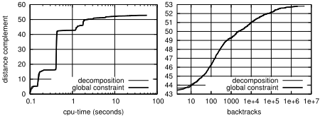
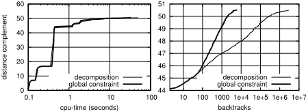
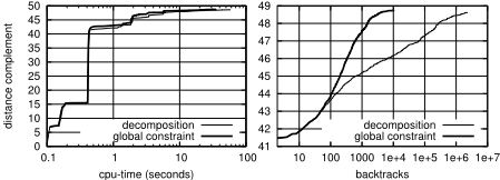
We compared the decomposition of distance constraints on each ideal separately as well as our propagation algorithm approximating GAC (Algorithm 3) for the combined distance global constraint. We report the results obtained in Figures 2(a), 2(b) and 2(c) for 2, 3 and 4 ideals, respectively.
1 ftp://ftp.irit.fr/pub/IRIT/RPDMP/Configuration
We plot n minus distance (the distance complement) against cpu-time, measured in seconds, and number of backtracks averaged over the 100 instances, in each case. More formally, we plot the following function, where St is the set of solutions found at time (or number of backtracks) t, V is the set of ideals and n is the number of variables:
Our search strategy was to chose the next variable to branch on with the usual domain/degree heuristic. The first value assigned was chosen so as to minimise the number of discrepancies with the ideals for its coordinate. In other words, given k vectors {v1, . . . , vk}, we choose for a variable Xi the value w ∈ D(Xi) such that ∑j∈[1,...,k] δj(w, vj[i]) was minimal.
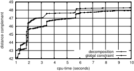
(d) A "zoom" on Figure 2(c).
Figure 2: Results for the Renault configuration problem.
On this benchmark the gain achieved in runtime using the global constraint instead of the decomposition is slight. Indeed, the curves are almost equal regardless of the number of
(c) Random instances: 4 ideals
Figure 3: Experimental results for the random instances.
ideals used. The optimal solution is often found very quickly, independent of the method used. In fact, the first solution is always found without backtracking, but since the problem is large there is a time penalty associated with finding it.
The logarithmic scale used to present cpu-time tends to hide the difference in time. In Figure 2(d) we "zoom" in on part of Figure 2(c), to show there is a reduction in cpu-time with the global constraint. We see that the global constraint achieves a distance complement of 47 in almost half the time taken by the decomposition.
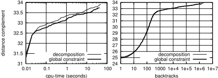
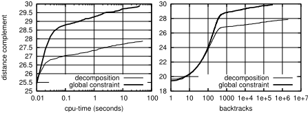
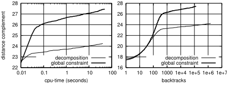
We also ran experiments on uniform binary random CSPs so that we could control how hard it is to achieve optimality, and hence we avoid the earlier situation where optimal solutions were found too easily. All instances have 100 variables, domain size is 10, and there are 250 binary constraints with a tightness of 0.3. These instance are thus underconstrained to allow for a sufficiently large set of solutions. They were generated using a random uniform CSP generator 2 . We generated 3 sets of 100 instances, with results presented in Figures 3(a), 3(b) and 3(c), for 2, 3, and 4 ideals, respectively. The improvement, both in runtime and number of backtracks, is seen as soon as the number of ideals exceeds 2. The cpu time overhead due to larger sets of ideals was not as important as expected. The reduction in the search tree clearly compensates for the computational cost of a single call to the algorithm.
2 http://www.lirmm.fr/˜bessiere/generator.html
8 RelatedWork
Constraints are not typically placed between the two solutions. One exception is the MAX-HAMMING problem where we seek a pair of solutions such that the Hamming distance between them is maximised [Angelsmark and Thapper, 2004], without the freedom to specify one of the solutions. In DISTANCE-SAT we seek solutions within some distance of each other [Bailleux and Marquis, 1999], which our work generalises in three important ways. First, we allow optimisation of the distances rather that stating a bound on distance. Second, we permit multiple ideals, and not just one. Third, we allow complex logical combinations of (non)ideals. Global constraints for reasoning about pair-wise distances between variables rather than between solutions, as proposed here, have also been proposed [Artiouchine and Baptiste, 2005; R´egin and Rueher, 2000].
9 Conclusion
We have proposed an approach to representing and reasoning about preferences in CSPs specified in terms of ideal and non-ideal solutions. We presented a novel global constraint for propagating distance constraints, which works with any distance metric that is component-wise decomposable like Hamming distance. Results from experiments with both realworld and random problem instances are encouraging.
Acknowledgements. Hebrard and O'Sullivan are supported by Science Foundation Ireland (Grant 00/PI.1/C075). Walsh is supported by NICTA, which is funded through the Australian Government's Backing Australia's Ability initiative, in part through the Australian Research Council.
@inproceedings{ijcai2007p15,
  title     = {Distance Constraints in Constraint Satisfaction},
  author    = {Hebrard, Emmanuel and O'Sullivan, Barry and Walsh, Toby},
  booktitle = {Proceedings of the Twentieth International Joint Conference on
               Artificial Intelligence, {IJCAI-07}},
  publisher = {International Joint Conferences on Artificial Intelligence},
  editor    = {Manuela M. Veloso},
  pages     = {106--110},
  year      = {2007},
  url       = {https://ijcai.org/proceedings/2007/15},
}
TY - CPAPER TI - Distance Constraints in Constraint Satisfaction AU - Hebrard, Emmanuel AU - O'Sullivan, Barry AU - Walsh, Toby T2 - Proceedings of the Twentieth International Joint Conference on Artificial Intelligence, IJCAI-07 PB - International Joint Conferences on Artificial Intelligence PY - 2007 SP - 106 EP - 110 UR - https://ijcai.org/proceedings/2007/15 ER -Copied
Machine-readable versions of this paper, for tools and AI agents:





