Learning Restart Strategies

1 Introduction

When trying to communicate across a lossy communication channel with unbounded delays, how long should we wait before resending an unanswered message? In multimodal function optimization using gradient descent, how many steps should we take before starting from a new random initial point? In randomized search over a tree, how deep should we go before abandoning all hopes of finding the goal, and starting the search anew? In similar situations, it is desirable to minimize the time to solve a given problem instance, with a given algorithm, whose run-time is a random variable with a possibly unknown distribution. A restart strategy can be used, to generate a sequence of "cutoff" times, at which the algorithm is restarted if unsuccessful.

It has been proved that knowledge of the run-time distribution (RTD) for a given algorithm/problem combination 1 can be used to determine an optimal uniform strategy, based on a constant cutoff [Luby et al., 1993]. In the same paper, the authors argue that such a strategy is of little practical interest, as a model of performance is usually unavailable. They then present a universal restart strategy, whose performance is worse than the optimal strategy by a logarithmic factor.

1 In the following, for the sake of readability, we will often refer to the RTD of a problem instance, meaning the RTD of different runs of the randomized algorithm of interest on that instance; and the RTD of a problem set, meaning the RTD of different runs of the randomized algorithm of interest, each run on a different instance,

These two strategies are based on opposite hypotheses about the availability of the RTD. As a third alternative, a runtime sample for a set of problem instances could be collected, and used to learn a model of the underlying RTD. There are two potential obstacles to this approach. First, gathering a meaningful sample of run-time data can be computationally expensive, especially in the very case where a restart strategy would be most useful, i. e., when the run-time exhibits huge variations [Gomes et al., 2000]. Second, a given problem set might contain instances with significantly different RTDs: the obtained model would capture the overall behavior of the algorithm on the set, but the corresponding restart strategy would be suboptimal for each instance. Problems met after the initial training phase could also be captured poorly by the estimated RTD, again leading to a suboptimal strategy.

Both obstacles are not difficult to circumvent. Training cost can be reduced by using a small censored sample of run-time values, obtained aborting runs that exceed some cutoff time. This obviously has an impact on the model's precision, but, the requirements in this sense are less strict than one would expect, and a coarse model already allows to evaluate a near-optimal strategy [Gagliolo and Schmidhuber, 2006b]. The second problem is unavoidable in a worst case setting; but in practical situations we do not expect the RTD of each instance of a problem set to be uncorrelated, and a sub-optimal uniform strategy based on the set RTD can still have a great advantage over the large bound of the universal.

In this paper we show how Luby's universal and uniform restart can be effectively interleaved, to solve a set of problem instances. The uniform strategy is based on a non-parametric model of the RTD on the problem set, which is updated every time a new problem instance is solved, in an online fashion. The resulting exploration vs. exploitation tradeoff, is treated as a bandit problem: a solver from [Auer et al., 1995] is used to allocate runs among the two strategies, such that, as the model converges, the uniform strategy is favored if the RTD

uniform randomly picked without replacement from the set.

of the set is close to the RTD of most instances, and worstcase bounds on performance are preserved otherwise.

In the following, restart strategies (Sect. 2) are briefly introduced, followed by a discussion of an "adversarial bandit" approach to algorithm selection (Sect. 3), which will be used in our strategy (Sect. 4). We give references to other related work in Sect. 5. Sect. 6 presents experiments with a randomized satisfiability problem solver. Sect. 7 discusses potential impact, and viable improvements, of the presented approach.

2 Optimal restart strategies

A restart strategy consists in executing a sequence of runs of a randomized algorithm, in order to solve a same problem instance, stopping each run r after a time T(r) if no solution is found, and restarting the algorithm with a different random seed; it can be operationally defined by a function T : N→R+ producing the sequence of thresholds T(r) employed. Luby et al. [1993] proved that the optimal restart strategy is uniform, i. e. , one in which a constant T(r) = T is used to bound each run. They show that in this case the expected value of the total run-time tT can be evaluated as

where F(t) is the cumulative distribution function (CDF) of the run-time for an unbounded run of the algorithm, i. e., a function quantifying the probability that the problem is solved before time t.

If such distribution is known, an optimal cutoff time T ∗ can be evaluated minimizing (1). Otherwise, the authors suggest a universal non-uniform restart strategy, with cutoff sequence {1, 1, 2, 1, 1, 2, 4, 1, ...}, 2 proving that its performance tU is bounded with high probability with respect to the expected run-time E(tT ∗ ) of the optimal uniform strategy, as

3 Algorithm selection as a bandit problem

Consider now a sequence B = {b1, ..., bM} of problem instances, and a set of algorithms A = {a1, a2, ..., aK}, such that each bm is solvable by at least one ak. Without loss of generality, we assume that the execution of each ak can be subdivided in sequential steps, and indicate with tk(r), r = 1, 2, ..., the duration of the r-th step of the k-th algorithm on the current problem. Each ak has its own mechanism for determining tk(r): e. g., for an iterative algorithm, tk(r) can be the cost of the r-th loop . In this setting, one generally wants to solve the incoming problem instances as fast as possible. This could mean identifying the single best algorithm for the whole set, or for each instance (algorithm selection [Rice, 1976]); or, in the more general setting of algorithm portfolios [Huberman et al., 1997], the optimal schedule for interleaving the execution of different algorithms, each performing well on different subsets of B.

2 The sequence is composed of powers of 2: when 2j-1 is used twice 2j is the next. More precisely, r = 1, 2, ..., T(r) := 2j-1 if r = 2j - 1; T(r) := T (r - 2j-1 + 1) if 2j-1 ≤ r < 2j - 1

In both cases, an obvious trade-off is faced, between exploration of the performance of the various ak, and exploitation of the solver(s) estimated to be fastest. A well-known, and well aged, paradigm for addressing such a trade-off is the multi-armed bandit problem. In its most basic form [Robbins, 1952], it is faced by a greedy gambler, playing a sequence of trials against a K-armed slot machine, each trial consisting of a choice of one of K available arms, whose rewards are randomly generated from different stationary distributions. The gambler can then receive the corresponding reward, and regret what he would have gained, if only he had pulled any of the other arms. The aim of the game is to minimize this regret, defined as the difference between the expected cumulative reward of the best arm, and the one cashed in by the gambler. Generally speaking, a bandit problem solver (BPS) can be described as a mapping from the entire history of observed rewards xk for each arm k to a probability distribution p = (p1, ..., pK), from which the choice for the successive trial is picked.

In recent works, the original restricting assumptions have been progressively relaxed. In the partial information case, only the reward of the pulled arm is revealed to the gambler. In the non-oblivious adversarial setting, the rewards for a given trial can be an arbitrary function of the entire history of the game, and are thus allowed to be deceptive, but have to be set before the current choice is made. Based on these pessimistic hypotheses, Auer et al. [1995] devised a probabilistic gambling scheme (Exp3), whose regret on a finite number of trials is bounded with high probability as O(M 2/3 (K log K)1/3 ), K being the number of arms, M the number of trials (see Alg. 1). The algorithm features a fixed lower bound γ on the exploration probability, and a parameter α controlling the amount of exploitation. Both can be set based on M to obtain the optimal regret rate above. 3

Algorithm 1 Exp3(M) by Auer et al.

set γ = min{1, ((K log K)/(2M))1/3} initialize sk := 0 for k = 1, ...,K; for each trial do set pk ∝ (1 + α)sk , ∑Kk=1 pk = 1 pick arm k with probability ˆ pk := (1 - γ)pk + γ/K observe reward xk ∈ [0, 1] update sk := sk + xkγ ˆ pkK

set α = ((4K log K)/M)1/3 end for

The selection of a best algorithm for a set of problems can be naturally described in a K-armed bandit setting, 4 where

3 The original formulation is based on a finite upper bound g on the cumulative reward of the best arm, which is at most M as each reward is in [0, 1]. A variant (Exp3.1) of the algorithm is proposed if M is unknown. The authors also present a better bound on the expected reward.

4 The cases of selection on an per-instance basis, and of algorithm portfolios, are more difficult to treat: bandit problem solvers usually provide bounds on regret with respect to a single arm, but the best algorithmmight be different for each problem.

"pick arm k" means "execute the next step of algorithm ak" (Alg. 2).

Algorithm 2 Algorithm selection using BP S

initialize BPS, p. for each problem do set tk := 0, rk := 0, k = 1, ...,K repeat pick k ∼ p execute step rk + 1 of ak update timer rk := rk + 1, tk := tk + tk(rk) if problem solved then observe reward xk := 1/tk else observe reward xk := 0 end if update p = BP S(k, xk) until problem solved end for

Note that this simple scheme falls in the partial information, non-oblivious adversarial setting, as we only observe reward for successful algorithms, and this reward depends on previous choices: for example, if ak takes R steps to solve a problem, we will not see any reward for the first R - 1 pulls. Our adversary is not malevolent, but it can be deceptive, especially if the tk(r) vary among algorithms: 5 even so, any bounds on performance of BPS will hold, and given our definition of reward, the expected performance of (Alg. 2) will converge to the one of the best solver for the set of problems.

4 Mixing restart strategies

Traditional statistical tests assess the goodness of a model measuring the fit of the corresponding probability density function (pdf) along the whole spectrum of observed samples. In our case, the sole purpose of the model ˆ F of the RTD is to set up a restart strategy, in order to gain on future performance, so the only quantity of practical interest is the loss in performance induced by the mismatch of our model. In [Gagliolo and Schmidhuber, 2006b] we studied the impact of increasingly censored sampling 6 on the performance of an estimated uniform restart strategy. This impact is quite low, due to the fact that (1) depends only on the lower quantiles of the distribution: a rough model of F , obtained from a heavily censored sample from the lower portion of the time scale, suffices to evaluate a near-optimal strategy, allowing to reduce its training cost.

The practical implementation of such a technique requires some censoring strategy to limit the cost of solving the train-

5 Consider a situation in which a1 solves a problem in one step of time 10, and gets reward 0.1, while a2 would have solved the same problem with 10 steps of duration 0.1 each, scoring reward 1.

6 Censored sampling is a commonly used technique in lifetime distribution estimation (see, e. g., [Nelson, 1982]), which allows to reduce the duration of a sequence of experiments, simply aborting runs exceeding a time threshold. The information carried by these runs can still be used for modeling, both in the parametric and nonparametric settings.

ing instances. Assuming no a priori information about T ∗, an ideal candidate is the universal strategy of Luby (Sect 2), as it invests equal portions of run-time on a set of exponentially spaced restart thresholds. Note that the restart thresholds of unsuccessful runs can be exploited in the form of censored samples. Such a simple scheme would allow to keep the performance bound of the universal strategy during training, and use the gathered data to estimate ˆ F, and the corresponding strategy ˆ T , to be exploited for future problem instances. To limit the cost of learning, and allow exploitation of the model to start as soon as possible, we will instead adopt an online, or life-long learning approach. We will use the "bandit" algorithm selection scheme described in Sect. 3 at an upper level, to control allocation of computational resources. In this case, the arms are the two restart strategies, each generating a sequence of restart thresholds Tk(rk), to bound a same algorithm s; "pull arm k" simply means "start s on the current problem, with threshold Tk(rk)". If the problem is not solved, tk(rk) = Tk(rk), and xk := 0; if it is solved in a time ts <= Tk(rk), tk(rk) = ts, and a positive reward is observed.

Our strategy GAMBLER (Alg. 3) starts by solving the first problem using the universal strategy alone. After a problem instance is solved, the solution time of the successful run, and all the collected censored samples from the unsuccessful runs, can be used to update the estimate ˆ F, and evaluate a new ˆ T , to be used on next problem. To model F, we will use the non-parametric product-limit estimator by Kaplan and Meier [1958]. It guarantees large sample convergence to an arbitrary distribution, and can account for censored samples as well. The non-parametric form is particularly appealing, as it does not require any a-priori assumptions about the RTD, it is fast to update, and the resulting CDF is a step-wise function, which makes the evaluation of the integral in (1) inexpensive.

To use Exp3 as the BPS we only need to normalize the rewards. We can do so by setting a lower and upper bound on ts, tmin ≤ ts ≤ tmax. In order to limit the impact of this choice on the convergence rate of Exp3, we adopt a logarithmic reward scheme: upon solution of a problem during a restart with strategy k, rk := (log tmax - log tk)/(log tmax - log tmin), tk being the total time spent by strategy k on that problem, including unsuccesful runs. In this way 1 is the maximum reward, that would be obtained by a strategy that solved a problem in a time tmin. Note that the use of a logarithm allows to set tmin and tmax, respectively, to a very small and a very large value, such that only the knowledge of a very loose bound on ts is required. 7

Let us now analyze how the bound (2) combines with the optimal regret of Exp3. In the following, E(y) is the expected value of a random variable y, tk represents solution time of strategy k on a single problem, Rk the number of restarts performed, pk ∈ [0, 1] the probability of picking a restart strategy, and indices T ∗, U, ˆ T , will label quantities related to Algorithm 3 GAMBLER(M) restart strategy for algorithm s

7 Also, the bound is not required to hold: if we always set ts := max{ts, tmin}, Exp3 will not be able to discriminate among two algorithms that always have ts ≤ tmin but will otherwise work; if we always restart algorithms exceeding tmax, Exp3 will still work if F ∗ (tmax) > 0). In both cases we can keep xk ∈ [0, 1].

set tmin, tmax initialize Exp3(M), pU = 1. for each problem 1, ..., M do set tk := 0, rk := 0, k = 1, 2 repeat pick k ∼ p run s with cutoff Tk(rk + 1) update timer rk := rk+1, tk := tk+min{ts, Tk(rk)} if problem solved then observe reward xk := log tmax-log tk log tmax-log tmin else observe reward xk := 0 end if update p =Exp3(k, xk) until problem solved end for

the unknown optimal uniform, universal, and estimated optimal uniform strategies, respectively, while G will identify our novel strategy GAMBLER, interleaving the execution of the latter two. On a given problem, for which the RTD of our algorithm s is F(t), a restart strategy with thresholds T (r) can be viewed as sequence of independent Bernoulli processes, with success probabilities F(T(r)). The number of restarts R required to solve the problem is then distributed with pdf p(R) = ∏R-1 r=1 (1 -F(T(r)))F(T(R)): for a uniform strategy T (r) = T , p(RT ) is geometric, with E(RT ) = 1/F (T ). For any deterministic strategy, the expected time to solve a problem is ET (r)(t) = ∑E(R) r=1 T(r), a monotonic function of E(R). For U this implies that the bound (2) can be translated into a bound on RU, with the same high probability. Given our simple reward scheme Exp3 will keep a constant p = (pU , p ˆ T ) during solution of a single problem. Consider now the worst-case setting in which ˆ T is such that F( ˆ T ) = 0, i. e., the uniform restart ˆ T will never solve the problem. If U spends RU restarts, in the meantime another Rˆ T restarts will have been wasted on ˆ T , with E(R ˆ T ) = E(RU )(1 - pU )/pU . As Exp3 always keeps pU ≥ γ/2, the expected performance of GAMBLER on this problem will then be bounded by E(tU +RU ˆ T (2 - γ)/γ) with high probability, and upper bounds on tU and RU will also guarantee an upper bound on tG.

5 Originality and related work

Restart strategies are particularly effective if the RTD of the controlled algorithm exhibits "heavy" tails, , i. e., is Pareto for both very large and very small values of time. Such behavior is observed for backtracking search on structured underconstrained problems in [Hogg and Williams, 1994; Gomes et al., 2000], but also in other problem domains, such as computer networks, as in [van Moorsel and Wolter, 2004]. An alternative solution is to run multiple copies of the same algorithm in parallel (algorithm portfolios [Huberman et al., 1997; Gomes and Selman, 2001]). In [Luby et al., 1993], Luby presents parallel restart strategies, which represent the natural combination with the portfolio approach: its solution is not adaptive, as it simply consists in restarting each algorithm with the universal strategy U. The literature on metalearning and algorithm selection [Giraud-Carrier et al., 2004; Rice, 1976], algorithm portfolios [Huberman et al., 1997; Gomes and Selman, 2001], anytime algorithms [Boddy and Dean, 1994], provides many examples of the application of performance modeling to resource allocation. Most works in these field adopt a more traditional offline approach, in which run-time samples are collected during an often impractically long initial training phase, and the obtained model is used without further tuning on subsequently met problems. As discussed in the introduction, this also implies stronger assumptions about the representativeness of the training set, and does not guarantee upper bounds on execution time.

The Max K-armed bandit problem is a variation on the original formulation, in which the estimated reward is only updated for the arm obtaining the maximum reward value, on a set of plays. Solvers for this game are used in [Cicirello and Smith, 2005; Streeter and Smith, 2006] to maximize performance quality, on a single problem instance.

Allocation of resources is usually set before each problem instance solution, and possibly updated afterward. Dynamic approaches, in which feedback information from the algorithms is exploited to adapt resource allocation during problem solution, represent a notable recent trend. In [Lagoudakis and Littman, 2000; Petrik, 2005], algorithm selection is modeled as a reinforcement learning problem, a more general setting than the bandit problem proposed in (Sect. 3). Models of performance conditional on the dynamic state after a fixed execution time are used in [Kautz et al., 2002; Wu, 2006] to implement dynamic context-sensitive restart policies for SAT solvers: also in this case the main difference of our approach is the online learning setting. [Gagliolo and Schmidhuber, 2006a] present a heuristic dynamic online learning approach to resource allocation, in which a conditional model of performance is trained and progressively exploited during training.

6 Experiments

The experiments were conducted using Satz-Rand [Gomes et al., 2000], a version of Satz [Li and Anbulagan, 1997] in which random noise influences the choice of the branching variable. Satz is a modified version of the complete DPLL procedure, in which the choice of the variable on which to branch next follows an heuristic ordering based on first and second level unit propagation. Satz-rand differs in that, after the list is formed, the next variable to branch on is randomly picked among the top h fraction of the list. We present results with the heuristic starting from the most constrained variables, as suggested in [Li and Anbulagan, 1997], and noise parameter set to 0.4.

A benchmark from SATLIB was used, consisting of different sets of "morphed" graph-coloring problems [Gent et al., 1999]: each graph is composed of the set of common edges among two random graphs, plus fractions p and 1-p of the remaining edges for each graph, chosen as to form regular ring lattices. Each of the 9 problem sets contains 100 instances, generated with a logarithmic grid of 9 different values for the parameter p, from 20 to 2-8 , to which we henceforth refer with labels 0, ..., 8. Satz-Rand has an initialization cost which depends only on the size of the problem, which in this case is the same for all sets. This cost was found to be always bigger than 105. We then set tmin = 105, tmax = 1012 (about 100 minutes on our machine), and, to be fair with the universal strategy, we multiplied and shifted its TU(r) as tmin(1 + TU(r)). With M = 100, parameters of Exp3 are determined as α = 0.38, γ = 0.19.

Each experiment was repeated 20 times with different random seeds, and a different random order of the instances. For comparison purposes, we repeated the experiments running the original algorithm, without restarts (labeled S) and the universal strategy alone (U). To compare with the ideal performance of T ∗ , we evaluated, a posteriori for each run, the T that minimized the cost of the problem set (TL(set)), and the cost of each instance (TL(inst)), based on the actual runtime outcomes. Note that these can be different for each run, and their performances are lower bounds on the performances of the optimal T ∗ , evaluated from the unknown actual RTD of, respectively, the problem set, and each problem instance. 8 The difference of these two bounds is particularly interesting, as it is an indirect measure of the heterogeneity of the RTD of the instances in each set. To show the effect of a more heterogeneous problem set, we also run experiments with all the 900 instances grouped as a single set (labeled A in the graph; M = 900, α = 0.18, γ = 0.09), again randomly mixed. In figure 6 we present, for each set, the total computation time 9 for our mixture (G), and the comparison terms. Upper 95% confidence bounds are given, estimated on the 20 runs. Plots of the RTD and restart cost for each set can be found in [Gagliolo and Schmidhuber, 2006b].

The results are quite impressive, and further confirm that the estimated restart strategy ˆ T is not very sensitive to the fit of the model ˆ F. In a typical run, between 40% and 80% of the sample is censored, as there is only one uncensored runtime for each task; the fit of the model is visibly bad, and it is limited to the lower portion of the time scale, near or below ˆ T, but ˆ T itself quickly converges close enough to T ∗, giving a near-optimal strategy.

Problems in 0 are easy. Satz-rand solves all instances in a similar time, any larger T is an optimal restart value, i.e., restarts are never executed, and the performance of a single copy S is the same as the ones of the optimal restarts. Also our GAMBLER quickly learns that, while U has to reach this value for every problem, resulting in a five times worst performance. In problems 1 to 5 we see the effect of a heavy-tailed RTD. S solves each set with times between 1.6 × 1010 (1)

8 As E(tT∗) = minT{E(tT)} ≥ E(minT{tT}) = E(tL) in both cases.

9 As we are also conducting experiments with parallel portfolios of heterogeneous algorithms, and thus we need a common measure of time, we modified the original code of Satz-rand adding a counter, that is incremented at every loop in the code. The resulting time measure was consistent with the number of backtracks. All results reported are in these loop cycles: on a 2.4 GHz machine, 109 cycles take about one minute.

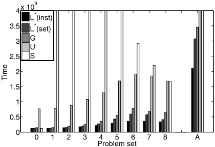
and 4.6 × 1012 (3). In practice, only a few "unlucky" runs have very long completion times, but this is enough to penalize its performance dramatically. GAMBLER scores fairly against the lower bounds, and U is between 3 and 5 times worst. From problem 6 on, we see that the heavy tail effect is less marked, but the two lower bounds diverge noticeably: instances in these sets present more heterogeneous RTDs, and the instance-optimal T ∗ (inst) may vary of more than one order of magnitude. Here U is only 2.5-3 times worse than GAMBLER. The worst performance of GAMBLER compared to L∗ (set) can be seen on problem 8, where tG is about 1.5 times tL∗ (set). Here most problems require a small threshold T , and a few require one about ten times larger: in this situation also threshold T ∗(set) varies visibly among different runs, and ˆ T sometimes overestimates the optimal threshold. Results on the whole set of problems A are better than expected: tG/tL∗ (set) is about 1.12, but the performance compared to tL∗ (inst) is obviously worst (1.65). This is natural, as both GAMBLER and T ∗(set) cannot discriminate different restarts for each problem. U completes the set at 1.17 × 109, about 3.4 times worse than GAMBLER.

7 Conclusions and future work

We presented a novel restart strategy (GAMBLER), combining the universal and optimal strategies by [Luby et al., 1993], based on a bandit approach to algorithm selection. GAMBLER takes the best of two worlds: it preserves the upper bounds of the universal strategy in a worst-case setting, and it proved to be effective in a realistic application, with only a small overhead over an ideal lower bound. It can save a few orders of magnitude in computation time for algorithms with a heavy-tailed RTD, and, unlike the universal strategy, it does not worsen the performance otherwise. It has a negligible overhead compared to the controlled algorithm, and does not require the tuning of any parameter, nor any a-prior assumption about the RTD, excluding very loose bounds on execution time, which in the presented experiments differed of 7 orders of magnitude. It does not require an initial training phase.

The parameters of Exp3 are automatically set based on the number of problems to be solved. If this number is not known in advance, Exp3.1 can be used instead.

The obtained strategy can be applied to any randomized algorithm, including, e. g., evolutionary algorithms, stochastic local search, gradient descent from a random initial value. Its main limitation is that it relies on the assumption that the problems to be solved display a similar RTD, but we saw in practice that this requirement is not strict, and the observed performance was consistently better than the one of the universal strategy alone.

The strategy has a modular structure: it would allow inclusion of more strategies, with an O(K logK) impact on performance, guaranteed by Exp3. Or more algorithms, each with its own RTD model. We particularly expect improvements from the use of conditional models, based on problem features, as they should allow for a distinction among different sub-classes of problems, sharing a similar RTD. A further step could be taken including dynamic information from the actual execution, as exemplified in [Kautz et al., 2002; Gagliolo and Schmidhuber, 2006a].

Acknowledgments. The authors would like to thank Faustino Gomez for precious comments on the draft of this paper. This work was supported by SNF grant 200020107590/1.