
Feature Selection Based on the Shapley Value
Proceedings of the Nineteenth International Joint Conference on Artificial Intelligence. Pages 665-669.
© 2005 International Joint Conferences on Artificial Intelligence
Abstract
We present and study the Contribution-Selection algorithm (CSA), a novel algorithm for feature selection. The algorithm is based on the Multiperturbation Shapley Analysis, a framework which relies on game theory to estimate usefulness. The algorithm iteratively estimates the usefulness of features and selects them accordingly, using either forward selection or backward elimination. Empirical comparison with several other existing feature selection methods shows that the backward elimination variant of CSA leads to the most accurate classification results on an array of datasets.
- [Alon et al., 1999] U. Alon, N. Barkai, D. A. Notterman, K. Gish, S. Ybarra, D. Mack, and A. J. Levine. Broad patterns of gene expression revealed by clustering of tu- mor and normal colon tissues probed by oligonucleotide arrays. Proc. Natl. Acad. Sci., 96:6745-6750, 1999.
- [Blake and Merz, 1998] C.L. Blake and C.J. Merz. UCI repository of machine learning databases. http://www.ics.uci.edu/ mlearn/MLRepository.html, 1998. University of California, Irvine, Dept. of Informa- tion and Computer Sciences. Link
- [Breiman, 2001] L. Breiman. Random forests. Machine Learning, 45(1):5-32, 2001.
- [Guyon, 2003] I. Guyon. Design of experiments for the NIPS 2003 variable selection benchmark. NIPS 2003 workshop on feature extraction and feature selection, 2003.
- [Joachims, 1999] T. Joachims. Making large-scale SVM learning practical. Advances in Kernel Methods -Support Vector Learning, B. Schlkopf and C. Burges and A. Smola (ed.), MIT-Press, 1999.
- [Keinan et al., 2004] A. Keinan, B. Sandbank, C. Hilgetag, I. Meilijson, and E. Ruppin. Fair attribution of functional contribution in artificial and biological networks. Neural Computation, 16(9), 2004.
- [Koller and Sahami, 1996] D. Koller and M. Sahami. To- ward optimal feature selection. Proceedings of the 13th In- ternational Conference on Machine Learning (ML), pages 284-292, 1996.
- [Perkins et al., 2003] S. Perkins, K. Lacker, and J. Theiler. Grafting: Fast, incremental feature selection by gradient descent in function space. Journal of Machine Learning Research, 3:1333-1356, 2003.
- [Shapley, 1953] L. S. Shapley. A value for n-person games. In H. W. Kuhn and A. W. Tucker, editors, Contributions to the Theory of Games, volume II of Annals of Mathemat- ics Studies 28, pages 307-317. Princeton University Press, Princeton, 1953.
References were extracted automatically from the PDF and may contain errors.
Full text extracted automatically from the PDF; figures, tables and equations may differ. The PDF is the version of record.
1 Introduction
Feature selection refers to the problem of selecting input variables, otherwise called features, that are relevant to predicting a target value for each instance in a dataset. Feature selection has several potential benefits: defying the curse of dimensionality to enhance the prediction performance, reducing measurement and storage requirements and reducing training and prediction times. This paper focuses on the first issue, namely selecting input variables in an attempt to maximize the performance of a classifier on previously unseen data.
In this paper, we suggest to recast the problem of feature selection in the context of coalitional games, a notion from game theory. This perspective yields an iterative algorithm for feature selection, the Contribution-Selection algorithm (CSA), intent on optimizing the performance of the classifier on unseen data. The algorithm combines both the filter and wrapper approaches. However, unlike filter methods, features are reranked on each step by using the classifier as a black box. The ranking is based on the Shapley value [Shapley, 1953], a well known concept from game theory, to estimate the importance of each feature for the task at hand, specifically taking into account interactions between features.
Throughout the paper we use the following notations. The distribution fromwhich the dataset instances are drawn is represented by two variables ✂ ✄ ✆ ✞ ✠ , where ✄ ☛ ✂ ✍ ✏ ✆ ✓ ✓ ✓ ✆ ✍ ✘ ✠ represents the input variables (vector of features), and ✞ represents a discrete target value (class) for ✄ . Three sets containing i.i.d. sampled instances of ✂ ✄ ✆ ✞ ✠ of the form ✢ ✣ ✤ ✆ ✦ ✤ ★ are available: Train, Validation and Test representing the training set, validation set and test set respectively. Given an induction algorithmand a set ✪ ✫ ✢ ✭ ✆ ✓ ✓ ✓ ✆ ✯ ★ , ✰ ✱ ✂ ✳ ✠ stands for a classifier constructed from the training set using the induction algorithm, after its input variables were narrowed down to the ones in S, namely ✰ ✱ ✂ ✳ ✠ labels each instance of the form ✂ ✳ ✶ ✷ ✆ ✓ ✓ ✓ ✳ ✶ ✻ ✼ ✻ ✠ , ✾ ✿ ❀ ✪ , ✭ ❃ ❅ ❃ ❈ ✪ ❈ with a value in the domain of ✞ . The task of feature selection is to choose a subset ✪ of the input variables, that would maximize the performance of the classifier on the test set. In what follows we shall focus on optimizing accuracy of the classifier, although we could as easily optimize other performance measure such as the area under the ROC curve, balanced error rate etc.
The rest of this paper is organized as follows: Section 2 introduces the necessary background from game theory with a detailed description of the CSA algorithm; Section 3 provides an empirical comparison of CSA with several other feature selection methods, accompanied by an analysis of the results; Section 4 discusses the empirical results and provides further insights to the success of the backward elimination version of the CSA algorithm.
2 Classification as a Coalitional Game
Cooperative game theory introduces the concept of "coalitional games", in which a set of players is associated with a payoff, a real function that denotes the benefit achieved by different sub-coalitions in a game. Formally, a coalitional game is defined by a pair ✂ ❊ ✆ ● ✠ where ❊ ☛ ✢ ✭ ✆ ✓ ✓ ✓ ✆ ✯ ★ is the set of all players and ● ✂ ✪ ✠ , for every ✪ ✫ ❊ , is a real number associating a worth with the coalition ✪ . Game theory further pursues the question of representing the contribution of each player to the game by constructing a value function, which assigns a real-value to each player. The values correspond to the contribution of the players in achieving a high payoff.
The contribution value calculation is based on the Shapley value [Shapley, 1953]. An intuitive example of the potential use of the Shapley value can be provided in an academic setting. Assume that you are a Professor running a lab, and, once and for all, you have decided to distribute the yearly bonus to your students in a fair manner, that reflects the actual contribution of each student to the academic success of the lab. During the year, the students form spontaneous "coalitions" of groups of students, each such group works and publishes a paper summarizing its work (these coalitions may also be assembled by the Professor). Every paper gets a rank, (e.g., its impact factor), composing its "payoff function". Based on this annual data of the students' coalitions and their associated payoffs, the Shapley value provides a fair and efficient way to distribute the bonus to each individual student according to his contribution over the year.
The Shapley value is defined as follows. Let the marginal importance of player ✾ to a coalition ✪ , with ✾ a0 ❀ ✪ , be
Then, the Shapley value is defined by the payoff
where ✒ is the set of permutations over ❊ , and ✪ ✶ ✂ ✏ ✠ is the set of players appearing before the ✾ th player in permutation ✏ . The Shapley value of a player is a weighted mean of its marginal value, averaged over all possible subsets of players.
Transforming these game theory concepts into the arena of feature selection, in which one attempts at estimating the contribution of each feature in generating a classifier, the players ❊ are mapped to the features of a dataset and the payoff is represented by a real-valued function ● ✂ ✪ ✠ , which measures the performance of a classifier generated using the set of features ✪ . Finally, the usage of the Shapley value for feature selection may be justified by its axiomatic qualities:
In the context of feature selection, this axiom implies that the performance on the dataset is divided fully between the different features.
Axiom 2 (Permutation invariance or symmetry) For any ✂ ❊ ✆ ● ✠ and permutation ✏ on ❊ it holds that ✞ ✶ ✂ ● ✠ ☛ ✞ ☛ ✖ ✶ ✘ ✂ ✏ ● ✠
This axiom implies that the value is not altered by arbitrarily renaming or reordering the features.
Axiom 3 (Preservation of carrier or dummy-property) For any game ✂ ❊ ✆ ● ✠ such that ● ✂ ✪ ✄ ✢ ✾ ★ ✠ ☛ ● ✂ ✪ ✠ for every ✪ ✫ ❊ it holds that ✞ ✶ ✂ ● ✠ ☛ ✛
This axiom implies that a dummy feature that does not influence the classifier's performance indeed receives a contribution value 0.
Axiom 4 (Additivity or aggregation) For any two games ✂ ❊ ✆ ● ✠ and ✂ ❊ ✆ ✢ ✠ it holds that ✞ ✶ ✂ ● ✤ ✢ ✠ ☛ ✞ ✶ ✂ ● ✠ ✤ ✞ ✶ ✂ ✢ ✠ where ✂ ● ✤ ✢ ✠ ✂ ✪ ✠ ☛ ● ✂ ✪ ✠ ✤ ✢ ✂ ✪ ✠
This axiom applies to a combination of two different payoffs based on the same set of features. For a classification task these may be, for example, accuracy and area under the ROC curve or false positive rate and false negative rate. In such case, the Shapley value of a feature, that measures its contribution to the combined performance measure, is just the sum of the corresponding Shapley values. The linearity of the Shapley value is a consequence of this property. Namely, if the payoff function ● is multiplied by a real number ✫ then all Shapley values are scaled by ✫ namely ✞ ✶ ✂ ✫ ● ✠ ☛ ✫ ✞ ✶ ✂ ● ✠ . In other words, multiplying the performance measure by a constant does not change the ranking of the features, a vital property for any scheme that ranks features by their 'importance'.
2.1 Estimating Features Contribution Using the MSA
The calculation of the Shapley value requires summing over all possible subsets of players, which is impractical in our case. [Keinan et al., 2004] have presented an unbiased estimator for the Shapley value by uniformly sampling permutations from ✒ . Still, the estimator considers both large and small features sets to calculate the contribution values. In our feature selection algorithm, we use the Shapley value heuristically to estimate the contribution value of a feature for the task of feature selection. Since in most realistic cases we assume that the size ✮ of significant interactions between features is much smaller than the number of features, ✯ , we will limit ourselves to calculating the contribution value from permutations sampled from the whole set of players, with ✮ being a bound on the permutation size. Notice that most filter methods are equivalent to using ✮ ☛ ✭ where no interactions are taken into account. Feature selection using Random Forests [Breiman, 2001] is equivalent to ✮ ✯ ✱ ✯ . The bounded estimated contribution value becomes
where ✒ ✴ is the set of sampled permutations on subsets of size ✮ . The usage of bounded sets coupled with the method for the Shapley value estimation, yields an efficient and robust way to estimate the contribution of a feature to the task of classification. For a detailed discussion of the MSA framework and its theoretical background see [Keinan et al., 2004].
2.2 The Contribution-Selection Algorithm
The Contribution-Selection algorithm (CSA), described in detail in Figure 1, is iterative in nature, and can either adopt a forward selection or backward elimination approach. Using the subroutine contribution, it ranks each feature according to its contribution value, and then selects ✶ features with the highest contribution values with forward selection (using the sub-routine selection) 1 , or eliminates ✷ features with the lowest contribution values with backward elimination (using elimination). It repeats the phases of calculating the contribution values of the remaining features given those already selected (or eliminated), and selecting (or eliminating) new features, until the contribution values of all candidate features
1 Alternatively, the selection sub-routine can use a forward selection technique instead of ✸ ; features are added in ascending order of their contribution values, as long as the classifier's performance improves.
- Contribution-Selection-Algorithm( a0 ; ✂ ✆ ✮ ✆ ✶ ) 1. ✶ ✷ ✁ ✷ ✄ ☎ ✷ ✮ := ✝ 2. for each ✰ ❀ a0 ✟ ✶ ✷ ✁ ✷ ✄ ☎ ✷ ✮ 2.1. ✡ ☛ := contribution(✰ , ✶ ✷ ✁ ✷ ✄ ☎ ✷ ✮ ; ✮ ) 3. if ✌ ✍ ✏ ☛ ✡ ☛ ✒ ✂ 3.1. ✶ ✷ ✁ ✷ ✄ ☎ ✷ ✮ := ✶ ✷ ✁ ✷ ✄ ☎ ✷ ✮ ✄ selection( ✢ ✡ ☛ ★ ; ✶ , ✂ ) 3.2. goto 2 else 3.3. return selected
Figure 1: The Contribution-Selection algorithm in its forward selection version. ✔ is the input set of features, ✕ is a contribution value threshold, ✖ is the maximal permutation size for calculating the contribution values, ✸ is the number of features selected in each phase. The contribution routine calculates the contribution value of feature ✗ with the pay off function described in this section. The selection routine selects at most ✸ features with highest contribution values that exceed ✕ . In the backward elimination version, the selection sub-routine is replaced with an elimination sub-routine which eliminates ✘ features in each phase and the halting criterion is changed accordingly.
exceed a contribution threshold ✂ with forward selection (or fall below a contribution threshold ✂ with backward elimination).
The algorithm, without further specification of the contribution sub-routine, is a generalization of filter methods. However, the main idea of the algorithm is that the contribution sub-routine, unlike common filter methods, returns a contribution value for each feature according to its assistance in improving the classifier's performance, which is generated using a specific induction algorithm, and in conjunction with other features. Using the notation in Section 2 and assuming one optimizes the accuracy level of the classifier, the contribution sub-routine for forward selection calculates the contribution values using the following payoff function ● ✂ ✪ ✠ :
- ✪ := ✪ ✄ ✶ ✷ ✁ ✷ ✄ ☎ ✷ ✮
- Generate a classifier ✰ ✱ ✂ ✳ ✠ from the training set, Train
- Evaluate ✰ ✱ ✂ ✳ ✠ for all examples of the validation set, Validation
- Return the accuracy level, defined as ● ✂ ✪ ✠ ☛ ✙ ✚ ✛ ✙ ☛ ✼ ✖ ✛ ✘ ✣ ✥ ✧ ✖ ✛ ✧ ✥ ✘ ☞ ✩ ✪ ✫ ✶ ✴ ✪ ✭ ✶ ✮ ✘ ✰ ✙ ✙ ✩ ✪ ✫ ✶ ✴ ✪ ✭ ✶ ✮ ✘ ✙
The case ✪ ☛ ✝ is an end case which is handled by returning the number of instances in the largest class divided by the total number of instances (a classifier which always selects the most frequent class). Backward elimination is quite similar, and the payoff is calculated by sampling permutations from the set of features left after each phase of elimination. The maximal permutation size ✮ has an important role in deciding the contribution values of the different features, and should be selected in a way that ensures that different combinations of features that interact together are inspected. Its impact is demonstrated in Section 3.
The number of selected features ✶ for the selection subroutine controls the redundancies of the selected features; the higher ✶ is, the more likely that features with redundant contribution will be selected. Although ✶ ☛ ✭ minimizes the redundancy dependencies of the features, increasing ✶ accelerates the algorithm's convergence. The algorithm's halting criterion depends on ✂ , which designates a trade-off between the number of selected features, and the performance of the classifier on the validation set. With the forward selection version, choosing ✂ ☛ ✛ means that CSA selects features as long as there exists a feature that is likely to improve the classifier's performance, and selects smaller sets of features as ✂ is increased. Increasing ✂ has the opposite effect on the size of the final set of features. The more intuitive halting criterion, to stop when no further performance gain is achieved, is too restrictive, while CSA's halting criterion enables the selection of features proved useful at later stages, as verified empirically over several datasets.
| Name | Classes | Features | Train Size | Test Size |
|---|---|---|---|---|
| Reuters1 | 3 | 1579 | 145 | 145 |
| Reuters2 | 3 | 1587 | 164 | 164 |
| Arrhythmia | 2 | 278 | 280 | 140 |
| Internet Ads | 2 | 1558 | 2200 | 800 |
| Dexter | 2 | 20000 | 300 | 300 |
| Arcene | 2 | 10000 | 100 | 100 |
| I2000 | 2 | 2000 | 40 | 22 |
3 Results
3.1 The Data and Benchmark Algorithms
To test CSA empirically we ran a number of experiments on seven real-world datasets with number of features ranging from 278 to 20,000 (Table 1): the Reuters1 dataset and the Reuters2 dataset both constructed following [Koller and Sahami, 1996] using the Reuters-21578 document collection; the Arrhythmia database from the UCI repository [Perkins et al., 2003] ; the Internet Advertisements database from the UCI repository [Blake and Merz, 1998] which was collected for the research of identifying advertisements in web pages, the Dexter text categorization dataset and the Arcene cancer dataset, both from the NIPS 2003 workshop on feature selection [Guyon, 2003] and the I2000 microarray colon cancer dataset [Alon et al., 1999].
In principle, CSA can work with any induction algorithm ✵ . However, due to computational constraints we focused on fast induction algorithms or algorithms that may be efficiently combined into CSA. We experimented with Naive Bayes, C4.5 and 1NN. For each of the datasets, we measured the training set accuracy of each classifier using ten-fold cross validation on the whole set features. For each dataset, all subsequent work used the induction algorithm ✵ , that gave the highest cross validation accuracy, as detailed in Table 2.
Eight different feature selection schemes were then compared on the datasets described above:
- ✶ The induction algorithm ✵ without performing feature selection to serve as a baseline.
- ✶ Regularized linear SVM using the ✪ ✷ ✹ ✫ ✶ ✻ ✽ ✭ package [Joachims, 1999]. Datasets that had more than two
| Dataset | L | ✶ (Fwd.) | ✷ (Bwd.) | ✮ | ☎ |
|---|---|---|---|---|---|
| Reuters1 | NB | 1 | 100 | 20 | 1500 |
| Reuters2 | NB | 1 | 100 | 20 | 1800 |
| Arrhythmia | C4.5 | 1 | 50 | 20 | 500 |
| Internet Ads | 1NN | 1 | 100 | 20 | 1500 |
| Dexter | C4.5 | 50 | 50 | 12 | 3500 |
| Arcene | C4.5 | 100 | 100 | 5 | 10000 |
| I2000 | C4.5 | 100 | 100 | 3 | 2000 |
classes were split into few binary classification problems.
- ✶ Filtering usingmutual information and classification using ✵ . We binned continuous domains to estimate the mutual information.
- ✶ Filtering using the Pearson correlation coefficient and classification using ✵ .
- ✶ Random Forests feature selection [Breiman, 2001] and classification using ✵ .
- ✶ Feature selection using forward selectionwrapper. Since simple wrapper greedily selects a feature that most improves the classifier's validation performance, it is equivalent to forward selection CSA with ✮ ☛ ✭ .
- ✶ Classification using ✵ after performing feature selection with forward selection CSA and parameters as described in Table 2. The parameters ✮ and ☎ were chosen such that the expected number of times that each feature is sampled is higher than 5. The contribution value threshold for stopping selection was ✂ ☛ ✛ . termination of feature selection was fixed by choosing a contribution value threshold ✂ ☛ ✛ . No hyperparameter selection was performed on either ✮ , ☎ or ✂ .
- ✶ Classification using ✵ after performing feature selection with backward elimination CSA and parameters as described in Table 2. The parameters ✮ and ☎ were chosen such that the expected number of times that each feature is sampled is higher than 5. The contribution value threshold for stopping elimination was ✂ ☛ ✛ . No hyperparameter selection was performed on either ✮ , ☎ or ✂
To avoid overfitting on the validation set used for calculating the payoff with CSA, we used m-fold cross validation instead of a single ✷ ✂ ✁ ✾ ✮ ✂ ☎ ✾ ✆ ✯ set.
3.2 Feature Selection and Classification Results
Table 3 summarizes the classifiers' performance on the test set and the number of features selected in each of the experiments. The accuracy levels are the fraction of correctly classified test set instances:
- ✶ The Reuters1 dataset. Feature selection using Random Forests did best, yielding accuracy level of 100% with 30 features. Not too far behind is the CSA in its backward elimination version (98.6% with 51 features). [Koller and Sahami, 1996], for example, report that the Markov Blanket algorithm yields approximately 600 selected features with accuracy levels of 95% to 96% on this dataset.
- ✶ The Reuters2 dataset. CSA with backward elimination did best, yielding accuracy level of 93% with 109 features. For comparison, [Koller and Sahami, 1996] report that the Markov Blanket algorithm yields approximately 600 selected features with accuracy levels of 89% to 93% on this dataset.
- ✶ The Arrhythmia dataset. This dataset is considered to be a difficult one. CSA with backward elimination did best, yielding an accuracy level of 84% with 21 features. Forward selection with higher depth value ( ✮ ☛ ✞ ✛ ) did better than wrapper, implying that one should consider many features concomitantly to perform good feature selection for this dataset. For comparison, the grafting algorithm [Perkins et al., 2003] yields an accuracy level of approximately 75% on this dataset.
- ✶ The Internet Ads dataset. All the algorithms did approximately the same, leading to accuracy levels between 94% and 96% with CSA slightly outperforming the others. Interestingly enough, the wrapper algorithm did not select any feature; in the first phase, the 1NN algorithm had neighbors from both classes with the same distance for each feature checked, leading to arbitrary selection of one of the classes, and the classifier's performance was constant through all the phase, yielding zero contribution values. However, when selecting the higher depth levels, the simple 1NN algorithm was boosted up to outperform classifiers such as SVM.
- ✶ The Dexter dataset. For the Dexter dataset, we used algorithm ✵ (C4.5 decision trees) only for the process of feature selection, and Linear SVM to perform the actual prediction on the features selected. This was done because C4.5 did not give satisfying accuracy levels for any of the feature selection algorithms, and it is impractical to use SVM with CSA for large datasets. To overcome the difference between the classifiers performing feature selection and the classifier used for the actual classification, we added an optimization phase for the forward selection algorithm after it stopped. In this phase, a ten-fold cross-validation is performed on the dataset in a similar way to the one used to optimize filter methods. The simple mutual information feature selection performed best, followed closely by the Contribution-Selection algorithm in its backward elimination version and by Random Forests. This implies that in Dexter the contribution of single features significantly outweigh the contribution of feature combinations for the task of classification. The forward selection algorithm did as well as Linear SVM without feature selection, but with a significantly lower number of features.
- ✶ The Arcene dataset. Here, just as in the case of Dexter, we use C4.5 for the process of feature selection, and Linear SVM to perform the actual prediction on the features
| Dataset | Wrapper | Fwd. | Bwd. | |
| Reuters1 | 92.4 (7) | 96.5 (10) | 98.6 (51) | |
| Reuters2 | 91.4 (5) | 90.1 (14) | 93.2 (109) | |
| Arrhythmia | 70 (5) | 74.2 (28) | 84.2 (21) | |
| Internet Ads | - | 95.6 (8) | 96.1 (158) | |
| Dexter | 80 (10) | 92.6 (100) | 93.3 (717) | |
| Arcene | 58 (7) | 81 (600) | 86 (7200) | |
| I2000 | 86.3 (550) | 86.3 (500) | 90.9 (1100) | |
| No FS | SVM Corr. | MI RF | ||
| 84.1 | 94.4 90.3 (20) | 94.4 (20) 100 (30) | ||
| 81.1 | 91.4 88.4 (20) | 90.2 (5) 87.2 (21) | ||
| 76.4 | 80 71.4 (20) | 70 (20) 80 (40) | ||
| 94.7 | 93.5 94.2 (15) | 95.75 (70) 95.6 (10) | ||
| 92.6 | 92.6 92.6 (1240) | 94 (230) 93.3 (800) | ||
| 83 | 83 83% (6600) | 81 (5600) 82 (6000) | ||
| 86.3 | 72.7 81.8 (260) | 90.9 (1060) 86.3 (100) | ||
selected. The CSA with backward elimination obtained better performance than the rest of the algorithms.
- ✶ The I2000 dataset. CSA with backward elimination and feature selection using mutual information yielded the best results. The poor performance of CSA with forward selection can be explained by the poverty of data comparing to the number of features; the algorithm selected in the first phases features which explain well the training data by coincidence, and avoided from selecting features that truly contribution to the task of classification. This phenomenon is explained in portrait in Section 3.3.
In summary, in 5 out of the 7 datasets, CSA with backward elimination achieved the best results. In all other cases, CSA achieved the second best result.
3.3 ACloser Inspection of the Results
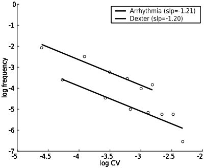
The MSA, intent on capturing correctly the contribution of elements to a task, enables us to examine the distribution of the contribution values of the features. Figure 2 depicts a log-log plot of the distribution of the contribution values in the first phase for Arrhythmia and Dexter, prior to making any feature selection. This distribution follows a scale-free power law, implying that large contribution values (in absolute value) are very rare, while small ones are quite common, justifying quantitatively the need of feature selection. The other datasets were also observed to possess similar power law characteristic.
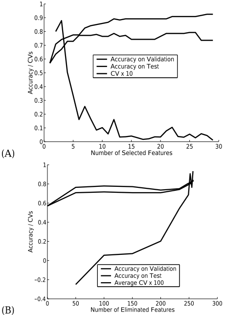
The behavior of the algorithm through the process of feature selection/elimination is displayed in Figure 3; after the forward selection algorithm identifies the significant features in the first few phases, there is a sharp decrease in the contribution values of the features selected in the following phases, while with backward elimination, there is a gradual and rather stable increase in the contribution values of the eliminated features. The peaks in the graph of the contribution values in Figure 3A demonstrate that the contribution values do change as the CSA iterates . In this case, the selection of a single feature considerably increased the contribution value of another feature, pointing at intricate dependencies between features.
Figures 2 and 3 also assist in explaining why backward elimination usually outperforms several feature selection methods, including forward selection; due to the high dimensionality of the datasets, a feature that assists in prediction merely by coincidence, may be selected, on the account of other truly informative features. Forward selection is penalized severely in such case: among the few significant features, some will not be chosen. However, backward elimination always maintains the significant features in the non eliminated set; a feature that truly enhances the classifier's generalization will do so for the validation set as well, and will not be eliminated. This leads to a more stable generalization behavior for backward elimination on the test set through the algorithm's progress (Figure 3).
4 Final Notes
The Contribution-Selection algorithm presented in this paper views the task of feature selection in the context of coalitional games. It uses a wrapper-like technique combined with a novel ranking method which is based on the Shapley contribution values of the features to the classification accuracy. The CSA works in an iterative manner, each time selecting new features (or eliminating them) while taking into account the features that were selected (or eliminated) so far.
CSA, similarly to wrapper algorithms, is restricted in the selection of the induction algorithm used for evaluating features sets, due to time limitations. This problem can be reduced by parallelizing, an advantage not shared by other wrapper algorithms which use search methods such as hill climbing; At each phase the permutations can be computed in parallel and upon completion combined to obtain an estimate of contribution values. Furthermore, as the algorithm progresses, the number of candidate features for either selection (forward selection) or elimination (backward elimination) decreases. Consequently, the number of permutations sampled may be reduced, speeding up the algorithm significantly. The restriction in selecting the learning algorithm for CSA does not apply to the prediction once the features are selected. After a set of features is found by the CSA, it may be used by any induction algorithm as demonstrated in section 3.2 with the Dexter and Arcene datasets.
We verified that the feature sets selected by CSA are significantly different than those selected by filter methods, and Random Forests. It turns out that the first "strong" features are selected by most methods. But within few iterations, filters and CSA select entirely different features due to the fact that the contribution values of the candidate features are modified, sometimes drastically, according to the already selected features.
The CSA was tested on number of datasets, and the results show that the algorithm can improve the performance of the classifier, and successfully compete with an existing array of feature selection methods, especially in cases where the features interact with each other; in such cases performing feature selection with a permutation size higher than one, namely not using the common greedy wrapper approach, can enhance the classifier's performance significantly.
The results successfully demonstrate the value of applying game theory concepts to feature selection. While the forward selection version of the algorithm is competitive with other feature selection methods, our experiments show that overall, the backward elimination version is superior to them, and produces features sets which can be used to generate a highly performing classifier.
@inproceedings{ijcai2005p76,
  title     = {Feature Selection Based on the Shapley Value},
  author    = {Cohen, Shay B. and Ruppin, Eytan and Dror, Gideon},
  booktitle = {Proceedings of the Nineteenth International Joint Conference on
               Artificial Intelligence, {IJCAI-05}},
  publisher = {International Joint Conferences on Artificial Intelligence},
  editor    = {Leslie Pack Kaelbling and Alessandro Saffiotti},
  pages     = {665--669},
  year      = {2005},
  url       = {https://ijcai.org/proceedings/2005/76},
}
TY - CPAPER TI - Feature Selection Based on the Shapley Value AU - Cohen, Shay B. AU - Ruppin, Eytan AU - Dror, Gideon T2 - Proceedings of the Nineteenth International Joint Conference on Artificial Intelligence, IJCAI-05 PB - International Joint Conferences on Artificial Intelligence PY - 2005 SP - 665 EP - 669 UR - https://ijcai.org/proceedings/2005/76 ER -Copied
Machine-readable versions of this paper, for tools and AI agents:





