
Semi-Supervised Regression with Co-Training
Proceedings of the Nineteenth International Joint Conference on Artificial Intelligence. Pages 908-915.
© 2005 International Joint Conferences on Artificial Intelligence
Abstract
In many practical machine learning and data mining applications, unlabeled training examples are readily available but labeled ones are fairly expensive to obtain. Therefore, semi-supervised learning algorithms such as co-training have attracted much attention. Previous research mainly focuses on semi-supervised classification. In this paper, a co-training style semi-supervised regression algorithm, i.e. COREG, is proposed. This algorithm uses two k-nearest neighbor regressors with different distance metrics, each of which labels the unlabeled data for the other regressor where the labeling confidence is estimated through consulting the influence of the labeling of unlabeled examples on the labeled ones. Experiments show that COREG can effectively exploit unlabeled data to improve regression estimates.
- [Blum and Chawla, 2001] A. Blum and S. Chawla. Learn- ing from labeled and unlabeled data using graph mincuts. In Proceedings of the 18th International Conference on Machine Learning, pages 19-26, Williamston, MA, 2001.
- Morgan Kaufmann. [Blum and Mitchell, 1998]
- A. Blum and T. Mitchell. Com- bining labeled and unlabeled data with co-training. In Proceedings of the 11th Annual Conference on Compu- tational Learning Theory, pages 92-100, Madison, WI, 1998. ACM Press.
- [Dasarathy, 1991] B. V. Dasarathy. Nearest Neighbor Norms: NN Pattern Classification Techniques. IEEE Com- puter Society Press, Los Alamitos, CA, 1991.
- [Dasgupta et al., 2002] S. Dasgupta, M. Littman, and D. McAllester. PAC generalization bounds for co-training. In T. G. Dietterich, S. Becker, and Z. Ghahramani, editors, Advances in Neural Information Processing Systems 14, pages 375-382. MIT Press, Cambridge, MA, 2002.
- [Dempster et al., 1977] A. P. Dempster, N. M. Laird, and D. B. Rubin. Maximum likelihood from incomplete data via the EM algorithm. Journal of the Royal Statistical So- ciety, Series B, 39(1):1-38, 1977.
- [Goldman and Zhou, 2000] S. Goldman and Y. Zhou. En- hancing supervised learning with unlabeled data. In Pro- ceedings of the 17th International Conference on Machine Learning, pages 327-334, San Francisco, CA, 2000.
- Mor- gan Kaufmann. [Hwa et al., 2003]
- R. Hwa, M. Osborne, A. Sarkar, and M. Steedman. Corrected co-training for statistical parsers. In Working Notes of the ICML'03 Workshop on the Contin- uum from Labeled to Unlabeled Data in Machine Learning and Data Mining, Washington, DC, 2003.
- [Joachims, 1999] T. Joachims. Transductive inference for text classification using support vector machines. In Pro- ceedings of the 16th International Conference on Machine Learning, pages 200-209, Bled, Slovenia, 1999.
- Morgan Kaufmann.
- [Miller and Uyar, 1997] D. J. Miller and H. S. Uyar. A mix- ture of experts classifier with learning based on both la- belled and unlabelled data. In M. Mozer, M. I. Jordan, and T. Petsche, editors, Advances in Neural Information Pro- cessing Systems 9, pages 571-577. MIT Press, Cambridge, MA, 1997.
- [Nigam and Ghani, 2000] K. Nigam and R. Ghani. Analyz- ing the effectiveness and applicability of co-training. In Proceedings of the 9th ACM International Conference on Information and Knowledge Management, pages 86-93, Washington, DC, 2000. ACM Press.
- [Nigam et al., 2000] K. Nigam, A. K. McCallum, S. Thrun, and T. Mitchell. Text classification from labeled and un- labeled documents using EM. Machine Learning, 39(2- 3):103-134, 2000.
- [Pierce and Cardie, 2001] D. Pierce and C. Cardie. Limi- tations of co-training for natural language learning from large data sets. In Proceedings of the 2001 Conference on Empirical Methods in Natural Language Processing, pages 1-9, Pittsburgh, PA, 2001.
- [Sarkar, 2001] A. Sarkar. Applying co-training methods to statistical parsing. In Proceedings of the 2nd Annual Meet- ing of the North American Chapter of the Association for Computational Linguistics, pages 95-102, Pittsburgh, PA, 2001.
- [Shahshahani and Landgrebe, 1994] B. Shahshahani and D. Landgrebe. The effect of unlabeled samples in re- ducing the small sample size problem and mitigating the hughes phenomenon. IEEE Transactions on Geoscience and Remote Sensing, 32(5):1087-1095, 1994.
- [Steedman et al., 2003] M. Steedman, M. Osborne, A. Sarkar, S. Clark, R. Hwa, J. Hockenmaier, P. Ruhlen, S. Baker, and J. Crim. Bootstrapping statistical parsers from small data sets. In Proceedings of the 11th Con- ference on the European Chapter of the Association for Computational Linguistics, pages 331-338, Budapest, Hungary, 2003.
- [Zhou et al., 2002] Z.-H. Zhou, J. Wu, and W. Tang. Ensem- bling neural networks: many could be better than all. Ar- tificial Intelligence, 137(1-2):239-263, 2002.
References were extracted automatically from the PDF and may contain errors.
Full text extracted automatically from the PDF; figures, tables and equations may differ. The PDF is the version of record.
1 Introduction
In many practical machine learning and data mining applications such as web user profile analysis, unlabeled training examples are readily available but labeled ones are fairly expensive to obtain because they require human effort. Therefore, semi-supervised learning methods that exploit unlabeled examples in addition to labeled ones have attracted much attention.
Many current semi-supervised learning methods use a generative model for the classifier and employ ExpectationMaximization (EM) [Dempster et al., 1977] to model the label estimation or parameter estimation process. For example, mixture of Gaussians [Shahshahani and Landgrebe, 1994], mixture of experts [Miller and Uyar, 1997], and naive Bayes [Nigam et al., 2000] have been respectively used as the generative model, while EM is used to combine labeled and unlabeled data for classification. There are also many other methods such as using transductive inference for support vector machines to optimize performance on a specific test set [Joachims, 1999], constructing a graph on the examples such that the minimum cut on the graph yields an optimal labeling of the unlabeled examples according to certain optimization functions [Blum and Chawla, 2001], etc.
A prominent achievement in this area is the co-training paradigm proposed by Blum and Mitchell [1998], which trains two classifiers separately on two sufficient and redundant views, i.e. two attribute sets each of which is sufficient for learning and conditionally independent to the other given the class label, and uses the predictions of each classifier on unlabeled examples to augment the training set of the other.
Dasgupta et al. [2002] have shown that when the requirement of sufficient and redundant views is met, the co-trained classifiers could make few generalization errors by maximizing their agreement over the unlabeled data. Unfortunately, such a requirement can hardly be met in most scenarios. Goldman and Zhou [2000] proposed an algorithm which does not exploit attribute partition. This algorithm requires using two different supervised learning algorithms that partition the instance space into a set of equivalence classes, and employs cross validation technique to determine how to label the unlabeled examples and how to produce the final hypothesis. Although the requirement of sufficient and redundant views is quite strict, the co-training paradigm has already been used in many domains such as statistical parsing and noun phrase identification [Hwa et al., 2003][Pierce and Cardie, 2001][Sarkar, 2001][Steedman et al., 2003].
It is noteworthy that previous research mainly focuses on classification while regression remains almost untouched. In this paper, a co-training style semi-supervised regression algorithm named COREG, i.e. CO-training REGressors, is proposed. This algorithm employs two k-nearest neighbor (kNN) regressors, each of which labels the unlabeled data for the other during the learning process. In order to choose appropriate unlabeled examples to label, COREG estimates the labeling confidence through consulting the influence of the labeling of unlabeled examples on the labeled examples. The final prediction is made by averaging the regression estimates generated by both regressors. Since COREG utilizes different distance metrics instead of requiring sufficient and redundant views, its applicability is broad. Moreover, experimental results show that this algorithm can effectively exploit unlabeled data to improve regression estimates.
The rest of this paper is organized as follows. Section 2 proposes the COREG algorithm. Section 3 presents an analysis on the algorithm. Section 4 reports on the experimental results. Finally, Section 5 concludes and raises several issues for future work.
2 COREG
Let L = {(x1, y1), · · · , (x|L|, y|L|)} denote the labeled example set, where xi is the i-th instance described by d attributes, yi is its real-valued label, i.e. its expected realvalued output, and |L| is the number of labeled examples; let U denote the unlabeled data set, where the instances are also described by the d attributes, whose real-valued labels are unknown, and |U| is the number of unlabeled examples.
Two regressors, i.e. h1 and h2, are generated from L, each of which is then refined with the help of unlabeled examples that are labeled by the latest version of the other regressor. Here the kNN regressor [Dasarathy, 1991] is used as the base learner to instantiate h1 and h2, which labels a new instance through averaging the real-valued labels of its k-nearest neighboring examples.
The use of kNN regressor as the base learner is due to the following considerations. First, the regressors will be refined in each of many learning iterations. If neural networks or regression trees are used, then in each iteration the regressors have to be re-trained with the labeled examples in addition to the newly labeled ones, the computational load of which will be quite heavy. Since kNN is a lazy learning method which does not hold a separate training phase, the refinement of the kNN regressors can be efficiently realized. Second, in order to choose appropriate unlabeled examples to label, the labeling confidence should be estimated. In COREG the estimation utilizes the neighboring properties of the training examples, which can be easily coupled with the kNN regressors.
It is noteworthy that the initial regressors should be diverse because if they are identical, then for either regressor, the unlabeled examples labeled by the other regressor may be the same as these labeled by the regressor for itself. Thus, the algorithm degenerates to self-training [Nigam and Ghani, 2000] with a single learner. In the standard setting of cotraining, the use of sufficient and redundant views enables the learners be different. Previous research has also shown that even when there is no natural attribute partitions, if there are sufficient redundancy among the attributes then a fairly reasonable attribute partition will enable co-training to exhibit advantages [Nigam and Ghani, 2000]. While in the extended co-training algorithm which does not require sufficient and redundant views, the diversity among the learners is achieved through using different learning algorithms [Goldman and Zhou, 2000]. Since COREG does not assume sufficient and redundant views and different learning algorithms, the diversity of the regressors should be sought from other channels.
Here the diversity is achieved through utilizing different distance metrics. In fact, a key of kNN learner is how to determine the distances between different instances. The Minkowsky distance shown in Eq. 1 is usually used for this purpose. Note that different concrete distance metrics can be generated through setting different values to the distance order, p. Roughly speaking, the smaller the order, the more robust the resulting distance metric to data variations; while the bigger the order, the more sensitive the resulting distance metric to data variations. Therefore, the vicinities identified for a given instance may be different using the Minkowsky distance with different orders. Thus, the kNN regressors h1
and h2 can be diverse through instantiating them with different p values. Such a setting can also bring another profit, that is, since it is usually difficult to decide which p value is better for the concerned task, the functions of these regressors may be somewhat complementary to be combined.
In order to choose appropriate unlabeled examples to label, the labeling confidence should be estimated such that the most confidently labeled example can be identified. In classification this is relatively straightforward because when making classifications, many classifiers can also provide an estimated probability (or an approximation) for the classification, e.g. a Naive Bayes classifier returns the maximum posteriori hypothesis where the posterior probabilities can be used, a BP neural network classifier returns thresholded classification where the real-valued outputs can be used, etc. Therefore, the labeling confidence can be estimated through consulting the probabilities of the unlabeled examples being labeled to different classes. For example, suppose the probability of the instance a being classified to the classes c1 and c2 is 0.90 and 0.10, respectively, while that of the instance b is 0.60 and 0.40, respectively. Then the instance a is more confident to be labeled (to class c1).
Unfortunately, in regression there is no such estimated probability that can be used directly. This is because in contrast to classification where the number of class labels to be predicted is finite, the possible predictions in regression are infinite. Therefore, a key of COREG is the mechanism for estimating the labeling confidence.
Heuristically, the most confidently labeled example of a regressor should be with such a property, i.e. the error of the regressor on the labeled example set should decrease the most if the most confidently labeled example is utilized. In other words, the most confidently labeled example should be the one which makes the regressor most consistent with the labeled example set. Thus, the mean squared error (MSE) of the regressor on the labeled example set can be evaluated first. Then, the MSE of the regressor utilizing the information provided by (xu, ˆyu) can be evaluated on the labeled example set, where xu is an unlabeled instance while ˆyu is the real-valued label generated by the original regressor. Let ∆u denote the result of subtracting the latter MSE from the former MSE. Note that the number of ∆u to be estimated equals to the number of unlabeled examples. Finally, (xu, ˆyu) associated with the biggest positive ∆u can be regarded as the most confidently labeled example.
Since repeatedly measuring the MSE of the kNN regressor on the whole labeled example set in each iteration will be time-consuming, considering that kNN regressor mainly utilizes local information, COREG employs an approximation. That is, for each xu, COREG identifies its k-nearest neighboring labeled examples and uses them to compute the MSE. In detail, let Ω denote the set of k-nearest neighboring labeled examples of xu, then the most confidently labeled example is identified through maximizing the value of ∆xu in Eq. 2, where h denotes the original regressor while h′ denotes the
Table 1: Pseudo-code describing the COREG algorithm
ALGORITHM: COREG
refined regressor which has utilized the information provided by (xu, ˆyu). Note that ˆyu = h(xu).
The pseudo code of COREG is shown in Table 1, where the function kNN(Lj, k, pj) returns a kNN regressor on the labeled example set Lj , whose distance order is pi. The learning process stops when the maximum number of learning iterations, i.e. T, is reached, or there is no unlabeled example which is capable of reducing the MSE of any of the regressors on the labeled example set. According to Blum and Mitchell [1998]'s suggestion, a pool of unlabeled examples smaller than U is used. Note that in each iteration the unlabeled example chosen by h1 won't be chosen by h2, which is an extra mechanism for encouraging the diversity of the regressors. Thus, even when h1 and h2 are similar, the examples they label for each other will still be different.
3 Analysis
This section attempts to analyze whether the learning process of COREG can use the unlabeled examples to improve the regression estimates. In order to simplify the discussion, here the effect of the pool U ′ is not considered as in [Blum and Mitchell, 1998]. That is, the unlabeled examples are assumed as being picked from the unlabeled example set U directly.
In each learning iteration of COREG, for each unlabeled example xu, its k-nearest neighboring labeled examples are put into the set Ω. As mentioned before, the newly labeled example should make the regressor become more consistent with the labeled data set. Therefore, a criterion shown in Eq. 3 can be used to evaluate the goodness of xu, where h is the original regressor while h′ is the one refined with (xu, ˆyu). If the value of ∆u is positive, then utilizing (xu, ˆyu) is beneficial.
In the COREG algorithm, the unlabeled example which maximizes the value of ∆xu is picked to be labeled. Therefore, the question is, whether the unlabeled example chosen according to the maximization of ∆xu will result in a positive ∆u value or not.
First, assume that (xu, ˆyu) is among the k-nearest neighbors of some examples in Ω, and is not among the k-nearest neighbors of any other examples in L. In this case, it is obvious that utilizing (xu, ˆyu) will only change the regression estimates on the examples in Ω, therefore Eq. 3 becomes Eq. 4. Comparing Eqs. 2 with 4 it can be found that the maximization of ∆xu also results in the maximization of ∆u.
Second, assume that (xu, ˆyu) is not among the k-nearest neighbors of any example in Ω. In this case, the value of ∆xu is zero, therefore (xu, ˆyu) won't be chosen in COREG.
Third, assume that (xu, ˆyu) is among the k-nearest neighbors of some examples in Ω as well as some examples in L - Ω, and assume these examples in L - Ω are (x′1 , y′1 ), · · · , (x′m, y′m). Then Eq. 3 becomes Eq. 5.
Maximizing ∆xu will maximize the first sum term of Eq. 5, but whether it can enable ∆u be positive should also refer the second sum term. Unfortunately, the value of this sum term is difficult to be measured except that the neighboring relationships between all the labeled examples and (xu, ˆyu) are evaluated. Therefore, there may exist cases where the unlabeled example chosen according to the maximization of ∆xu may decrease ∆u, which is the cost COREG takes for using ∆xu that can be more efficiently computed to approximate ∆u. Nevertheless, experiments show that in most cases such an approximation is effective.
It seems that using only one regressor to label the unlabeled examples for itself might be feasible, where the unlabeled examples can be chosen according to the maximization of ∆xu .
While considering that the labeled example set usually contains noise, the use of two regressors can be helpful to reduce overfitting.
Let Λ denote the subset of noisy examples in L. For the unlabeled instance xu, either of the regressors h1 and h2 will identify a set of k-nearest neighboring labeled examples for xu. Assume these sets are Ω1 and Ω2, respectively. Since h1 and h2 use different distance orders, Ω1 and Ω2 are usually different, and therefore Ω1 ∩ Λ and Ω2 ∩ Λ are also usually different. Suppose xu is labeled by h1 and then (xu, h1(xu)) is put into L1, where h1(xu) suffers from Ω1 ∩ Λ. For another unlabeled instance xv which is very close to xu, its k-nearest neighbors identified by h1 will be very similar to Ω1 except that (xu, h1(xu)) has replaced a previous neighbor. Thus, h1(xv) will suffer from Ω1 ∩ Λ more seriously than h1(xu) does. While, if the instance xu is labeled by h2 and (xu, h2(xu)) is put into L1, then h1(xv) will suffer from Ω1 ∩ Λ only once, although xu is still very close to xv.
4 Experiments
Experiments are performed on ten data sets listed in Table 2 where "# attribute" denotes the number of input attributes. These data sets have been used in [Zhou et al., 2002] where the detailed descriptions of the data sets can be found. Note that the input attributes as well as the real-valued labels have been normalized to [0.0, 1.0].
| Data set | # attribute | Size |
|---|---|---|
| 2-d Mexican Hat | 1 | 5,000 |
| 3-d Mexican Hat | 2 | 3,000 |
| Friedman #1 | 5 | 5,000 |
| Friedman #2 | 4 | 5,000 |
| Friedman #3 | 4 | 3,000 |
| Gabor | 2 | 3,000 |
| Multi | 5 | 4,000 |
| Plane | 2 | 1,000 |
| Polynomial | 1 | 3,000 |
| SinC | 1 | 3,000 |
For each data set, 25% data are kept as the test set, while the remaining 75% data are partitioned into the labeled and unlabeled sets where 10% (of the 75%) data are used as labeled examples while the remaining 90% (of the 75%) data are used as unlabeled examples.
In the experiments, the distance orders used by the two kNN regressors in COREG are set to 2 and 5, respectively, the k value is set to 3, the maximum number of iterations T is set to 100, and the pool U ′ contains 100 unlabeled examples randomly picked from the unlabeled set in each iteration.
A self-training style algorithm is tested for comparison, which is denoted by SELF. This algorithm uses a kNN regressor and in each iteration, it chooses the unlabeled example which maximizes the value of ∆xu in Eq. 2 to label for itself. Moreover, a co-training style algorithm, denoted by ARTRE, is also tested. Since the experimental data sets are with no sufficient and redundant views, here an artificial redundant view is developed through deriving new attributes from the original ones. For example, on 3-d Mexican Hat two new attributes, i.e. x3 and x4, are constructed from x1 + x2 and x1 - x2, and then a kNN regressor is built on x1 and x2 while the other is built on x3 and x4. In each iteration, each kNN regressor chooses the unlabeled example which maximizes the value of ∆xu in Eq. 2 to label for the other regressor. The final prediction is made by averaging the regression estimates of these two refined regressors. Besides, a kNN regressor using only the labeled data is tested as a baseline for the comparison, which is denoted by LABELED.
All the kNN regressors used in SELF, ARTRE, and LABELED employ 2nd-order Minkowski distance, and the k value is set to 3. The same pool, U ′ , as that used by COREG is used in each iteration of SELF and ARTRE, and the maximum number of iterations is also set to 100.
One hundred runs of experiments are carried out on each data set. In each run, the performance of all the four algorithms, i.e. COREG, SELF, ARTRE, and LABELED, are evaluated on randomly partitioned labeled/unlabeled/test splits. The average MSE at each iteration is recorded. Note that the learning processes of the algorithms may stop before the maximum number of iterations is reached, and in that case, the final MSE is used in computing the average MSE of the following iterations.
The improvement on average MSE obtained by exploiting unlabeled examples is tabulated in Table 3, which is computed by subtracting the final MSE from the initial MSE and then divided by the initial MSE.
| Data set | SELF | ARTRE | COREG |
|---|---|---|---|
| 2d Mexican Hat | 9.2% | 12.8% | 19.6% |
| 3d Mexican Hat | 3.9% | 3.7% | 5.7% |
| Friedman #1 | -1.8% | -4.0% | 0.5% |
| Friedman #2 | -1.3% | -4.3% | 2.1% |
| Friedman #3 | -0.9% | -3.6% | 0.0% |
| Gabor | 4.0% | 3.8% | 9.0% |
| Multi | -1.9% | -4.4% | 1.4% |
| Plane | -3.8% | -3.5% | -1.6% |
| Polynomial | 15.1% | 17.4% | 22.0% |
| SinC | 13.0% | 16.4% | 26.0% |
Table 3 shows that SELF and ARTRE improve the regression estimates on only five data sets, while COREG improves on eight data sets. Moreover, Table 3 discloses that the improvement of COREG is always bigger than that of SELF and ARTRE. These observations tell that COREG can effectively exploit unlabeled examples to improve regression estimates.
For further studying the compared algorithms, the average MSE of different algorithms at different iterations are plotted in Fig 1, where the average MSE of the two kNN regressors used in COREG are also depicted. Note that in each subfigure, every curve contains 101 points corresponding to the 100 learning iterations in addition to the initial condition, where only 11 of them are explicitly depicted for better presentation.
Fig. 1 shows that COREG can exploit unlabeled examples to improve the regression estimates on most data sets, except that on Friedman #3 there is no improvement while on Plane the performance is degenerated. While, SELF and ARTRE degenerate the regression estimates on five data sets, i.e. Friedman #1 to #3, Multi, and Plane. Moreover, the average MSE of the final prediction made by COREG is almost always the best except on Friedman #1 where ARTRE is slightly better and on Plane where LABELED is the best while all the semisupervised learning algorithms degenerate the performance. These observations disclose that COREG is apparently the best algorithm in the comparison.
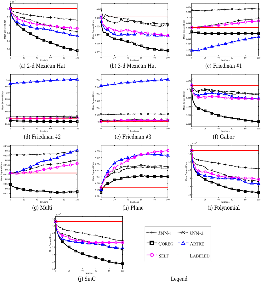
Pairwise two-tailed t-tests with 0.05 significance level reveal that the final regression estimates of COREG are significantly better than its initial regression estimates on almost all the data sets except that on Plane the latter is better while on Friedman #3 there is no significant difference. Moreover, the final regression estimates of COREG are significantly better than these of ARTRE on almost all the data sets except on Friedman #1 where the latter is better. Furthermore, the final regression estimates of COREG are significantly better than these of SELF and LABELED on almost all the data sets except on Plane where LABELED is better and on Friedman #3 where there is no significant difference. These results of t-tests confirm that COREG is the strongest among the compared algorithms, which can effectively exploit unlabeled data to improve the regression estimates.
5 Conclusion
This paper proposes a co-training style semi-supervised regression algorithm COREG. This algorithm employs two knearest neighbor regressors using different distance metrics. In each learning iteration, each regressor labels the unlabeled example which can be most confidently labeled for the other learner, where the labeling confidence is estimated through considering the consistency of the regressor with the labeled example set. The final prediction is made by averaging the predictions of both the refined kNN regressors. Experiments show that COREG can effectively exploit unlabeled data to improve the regression estimates.
In contrast to standard co-training setting, COREG does not require sufficient and redundant views, which enables it have broad applicability. However, this forces COREG generate diverse initial regressors with specific mechanisms. In this paper the diversity is obtained by instantiating the Minkowski distance with different distance orders. It is obvious that using completely different distance metrics may be more helpful. Moreover, trying to obtain the diversity of the initial regressors from channels other than using different distance metrics is an issue to be investigated in future work. Note that although this paper uses kNN regressor as the base learner, an important idea of COREG, i.e. regarding the labeling of the unlabeled example which makes the regressor most consistent with the labeled example set as with the most confidence, can also be used with other base learners. Therefore, designing semi-supervised regression algorithms with other base learners along the way of COREG is another interesting issue to be explored in the future. Furthermore, designing semi-supervised regression algorithms outside the co-training framework is also well-worth studying.
Acknowledgments
Supported by NSFC (60325207), FANEDD (200343), and JIANGSUSF (BK2004001).
@inproceedings{ijcai2005p66,
  title     = {Semi-Supervised Regression with Co-Training},
  author    = {Zhou, Zhi-Hua and Li, Ming},
  booktitle = {Proceedings of the Nineteenth International Joint Conference on
               Artificial Intelligence, {IJCAI-05}},
  publisher = {International Joint Conferences on Artificial Intelligence},
  editor    = {Leslie Pack Kaelbling and Alessandro Saffiotti},
  pages     = {908--915},
  year      = {2005},
  url       = {https://ijcai.org/proceedings/2005/66},
}
TY - CPAPER TI - Semi-Supervised Regression with Co-Training AU - Zhou, Zhi-Hua AU - Li, Ming T2 - Proceedings of the Nineteenth International Joint Conference on Artificial Intelligence, IJCAI-05 PB - International Joint Conferences on Artificial Intelligence PY - 2005 SP - 908 EP - 915 UR - https://ijcai.org/proceedings/2005/66 ER -Copied
Machine-readable versions of this paper, for tools and AI agents:





