
Signal-to-Score Music Transcription using Graphical Models
Proceedings of the Nineteenth International Joint Conference on Artificial Intelligence. Pages 758-764.
© 2005 International Joint Conferences on Artificial Intelligence
Abstract
We present a transcription system that takes a music signal as input and returns its musical score. Two stages of processing are used. The first employs a fundamental frequency detector and an onset detector to transform input signals into a sequence of sound events. The onset detection is inherently noisy. This paper focuses on the second stage, going from sound events to a notated score. We use a family of graphical models for this task. We allow the results of onset detection to be noisy, necessitating a search over possible segmentations of the sound events. We use a large corpus of monophonic vocal music to evaluate our system. Our results show that our approach is well-suited to the problem of music transcription. The initial onset detection reduces the number of observations and makes the system less instrument specific. The search over segmentations corrects the errors in the onset detection. Without such reasoning, these errors are magnified in subsequent rhythm transcription.
- [Cemgil and Kappen, 2003] Ali Taylan Cemgil and Bert Kappen. Monte Carlo methods for tempo tracking and rhythm quantization. Journal of Artificial Intelligence Re- search, 18:45-81, 2003.
- [Cemgil et al., 2004] Ali Taylan Cemgil, Bert Kappen, and David Barber. A generative model for music transcrip- tion. IEEE Transactions on Speech and Audio Processing, 2004.
- [Dixon, 2001] Simon Dixon. Automatic extraction of tempo and beat from expressive performances. Journal of the New Music Research, 30(1):39-58, 2001.
- [Gilks et al., 1996] W. R. Gilks, S. Richardson, and D. J. Spiegelhalter, editors. Markov Chain Monte Carlo in Practice. Chapman and Hall, London, 1996.
- [Goto and Muraoka, 1998] Masataka Goto and Yoichi Mu- raoka. An audio-based real-time beat tracking system and its applications. In Proceedings of the International Com- puter Music Conference, San Francisco, California, 1998.
- [Green, 1995] Peter J. Green. Reversible jump Markov chain Monte Carlo computation and Bayesian model determina- tion. Biometrika, 82:711-732, 1995.
- [Kapanci and Pfeffer, 2004] Emir Kapanci and Avi Pfeffer. A hierarchical approach to onset detection. In Proceedings of the International Computer Music Conference, Miami, Florida, 2004.
- [Klapuri, 2004] Anssi Klapuri. Signal Processing Methods for Automatic Transcription of Music. PhD thesis, Tam- pere University of Technology, Tampere, Finland, 2004.
- [Marolt, 2004] M. Marolt. A connectionist approach to tran- scription of polyphonic piano music. IEEE Transactions on Multimedia, 6(3):439-449, 2004.
- [Pasula and Russell, 2001] Hanna Pasula and Stuart Russell. Approximate inference for first-order probabilistic lan- guages. In Proceedings of the International Joint Confer- ence of Artificial Intelligence, Seattle, Washington, 2001. IJCAI
- [Platt, 1999] John C. Platt. Probabilistic outputs for support vector machines and comparisons to regularized likelihood methods. In A. J. Samola, P. Bartlett, B. Scholkopf, and D.Schuurmans, editors, Advances in Large Margin Classi- fiers, pages 185-208. MIT Press, Cambridge, MA, 1999.
- [Raphael, 2002a] Chris Raphael. Automatic transcription of piano music. In Proceedings of the International Sympo- sium on Music Information Retrieval, Paris, France, 2002.
- [Raphael, 2002b] Chris Raphael. A hybrid graphical model for rhythmic parsing. Artificial Intelligence, 137(1- 2):217-238, 2002.
- [Sterian, 1999] Andrew Sterian. Model-Based Segmenta- tion of Time-Frequency Images for Music Transcription. PhD thesis, University of Michigan, Ann Arbor, Michi- gan, 1999.
References were extracted automatically from the PDF and may contain errors.
Full text extracted automatically from the PDF; figures, tables and equations may differ. The PDF is the version of record.
1 Introduction
Music transcription is the task of transforming a music signal into a symbolic representation of the musical events it contains. There are three levels of representation of music that are relevant here. On the third level is the musical score in common music notation. This consists of musical events with attributes notated pitch (such as "A" in octave 4), notated duration (such as quarter note), and notated rhythmic position (such as the first beat of measure 22). On the second level is the representation of performance in terms of sound events. This is the level of MIDI data. The rhythmic attributes of events on this level are the actual onset time (such as 3.4 seconds from the beginning of the piece) and the actual duration (such as 0.5 seconds). The pitch attribute on this level could be discrete (such as MIDI note 66) or continuous (such as 66.46). On the first level is the representation of the sound signal. It is a common practice to transform the signal into a sequence of frames (through short-time Fourier transform), which are snapshots of the signal over a short period of time (e.g. 20 msecs). A frame captures the composition of the sound by specifying the amplitude for every frequency.
The third level is the target representation of transcription. Previous authors [Raphael, 2002b; Cemgil and Kappen, 2003] have proposed using graphical models for automated music transcription, but their systems take MIDI data as input and only go from the second to the third level. Our goal is to build an end-to-end transcription system that goes all the way from a first level audio signal to a third level musical score. In this work we focus on monophonic transcription from a complex instrument such as voice. Monophonic transcription is a difficult enough task, and well worthy of study. It raises many issues that need to be addressed before polyphonic transcription can be attempted. Going from level 1 to 3 is a much more challenging task than going from level 2 to 3. In going from level 2 to 3, there is a one-to-one mapping between musical events. Furthermore, the input is often MIDI data where the pitch is given and does not need to be detected. Therefore the only work that needs to be done is to track the tempo of the music, thereby transforming actual onset times and durations into notated rhythmic positions and durations.
Going from level 1 directly to level 3 is too hard. Frames are too small a unit and even short music signals will be represented by very long sequences of frames. Each musical event consists of many frames that need to be grouped together. Furthermore, the information in a frame needs to be summarized. Instead of a frequency-amplitude spectrum, we need to know the fundamental frequency of a given frame. Therefore we use a preprocessing step in which we go from level 1 to level 2. This step consists of a fundamental frequency detector, which determines the fundamental frequency sounding in each frame, and an onset detector, which detects the beginnings of musical events from the frame sequence. Once a musical event has been identified, an overall pitch for the event can be deduced by analyzing all the frames constituting the event. We have previously built an onset detector capable of handling the soft onsets prevalent in vocal music, in which there is a smooth pitch change, or a vowel change [Kapanci and Pfeffer, 2004]. While achieving state-of-the-art performance, it is not completely reliable, and no perfect onset detector exists. It might miss some onsets, causing it to merge musical events, while reporting other spurious onsets, causing it to separate events. Furthermore, the pitch data produced by the onset detector is continuous-valued and noisy.
This paper focuses on the transformation from level 2 to 3 when the level 2 input is noisy. We do not assume a one-toone mapping between events at the two levels. Instead, we allow for the possibility that reported onsets are false positives. The onset detector can be tuned to trade off the rate of false positives with false negatives. We use a setting with a very low false negative rate, so that most of the errors in onset detection are false positives. We also detect the pitch, allowing the tuning of the performance to change over time. So we need to simultaneously (1) detect false positives in the segmentation, (2) do tempo tracking and rhythm transcription, and (3) do tuning tracking and pitch transcription.
We propose a family of graphical models to accomplish these tasks. In the models, the properties of sound events depend probabilistically on the properties of notated events to which they are related. Because there may be false onsets, several sound events may actually be related to the same notated event. The segmentation determines which sound events are grouped together into a single note event, and therefore it determines the structure of the graphical model. We have a different graphical model corresponding to each possible segmentation. We use Markov Chain Monte Carlo (MCMC) sampling to search over the different structures and parameters.
We evaluate our model using a corpus of monophonic vocal music. Our results show that in the absence of perfect onset detectors, reasoning about segmentation is necessary for a signal-to-score system. Without such reasoning, the errors in the segmentation are magnified in subsequent rhythm transcription. We also show that the transcription benefits from musical knowledge, which is easily incorporated into our graphical model as prior distributions over the scores.
2 Problem Statement
The input of our system is a music signal, and the output is a musical score. The music signal is first processed using an onset detector to yield the sound event observations a0 ✁ ✄ ✆ for the graphical model. Each sound observation a0 ✝ consists of an observed duration ✟ ✝ and a frequency ✡ ✝ . The task is to find a segmentation ☞ ✁ ✄ ✍ and a score ✎ ✁ ✄ ✍ . Each score event ✎ ✑ consists of a notated duration ✓ ✑ and a pitch ✔ ✑ . The segmentation variable ☞ ✑ is the number of observed events related to the ✕ th score event. Thus the segmentation determines the mapping between score events and observed events. ✖ is the number of observations (fixed), while ✗ is the number of note events (dependent on the segmentation).
The goal is to find the segmentation ☞ ✁ ✄ ✍ and the score ✎ ✁ ✄ ✍ that maximize the posterior probability of the segmentation and score given the observed data:
assuming independence of the prior distributions over score and segmentation. The graphical model detailed in section 3 defines ✷ ✘ a0 ✁ ✄ ✆ ✺ ☞ ✁ ✄ ✍ ✙ ✎ ✁ ✄ ✍ ✛ . We have a style specific score prior ✷ ✘ ✎ ✁ ✄ ✍ ✛ , and a segmentation prior ✷ ✘ ☞ ✁ ✄ ✍ ✛ based on the onset detector's outputs. The output of the system is the score ✎ ✢ ✁ ✄ ✍ and the mapping of observations to the score events ☞ ✢ ✁ ✄ ✍ . We evaluate it using a metric presented in Section 5.
For our onset detector, we use our previously published hierarchical method that detects onsets in a signal by comparing frames one to another [Kapanci and Pfeffer, 2004]. A comparison function based on the fundamental frequencies and amplitudes returns the dissimilarity of two frames. If this value is above a threshold, an onset is declared over the region delimited by the two frames. The system begins by comparing adjacent frames, and then gradually increases the distance between the compared frames. By comparing frames some distance apart, the detector is able to detect soft onsets that happen smoothly over time.
To reduce the number of missed onsets, we use a low dissimilarity threshold. That way, we get many extraneous onsets (false positives) which need to be eliminated in later stages, but missed onsets (false negatives) are infrequent. In our experiments, 40% of the onsets were extraneous, while only 1.39% of the onsets were missed.
Once the onsets are marked, the signal is segmented by cutting it at these onsets. A continuous pitch attribute is computed for each event by the average fundamental frequency. The comparison value for each detected onset is also stored to be used in assigning a prior segmentation probability to each observation a0 ✝ , as described in the next section.
3 Model
The likelihood of a sequence of observed sound events is given by a family of graphical models. Due to the possibility of false onsets, there are many possible groupings of sound events (observations) into note events. The segmentation determines which sound events are grouped together, and therefore it determines the structure of the graphical model. For each segmentation ☞ ✁ ✄ ✍ , the likelihood model defines the probability of observations a0 ✁ ✄ ✆ ✣ ✘ ✟ ✁ ✄ ✆ ✙ ✡ ✁ ✄ ✆ ✛ given ✎ ✁ ✄ ✍ ✣ ✘ ✓ ✁ ✄ ✍ ✙ ✔ ✁ ✄ ✍ ✛ . The probabilistic dependency of sound events on the notated events is the same in different structures. The difference is in the connections between the two layers as illustrated in Figures 1 and 2: the leaf nodes correspond to the observations, and the segmentation determines the structure of the graph above them. The mapping between observation indexes (❇ s) and note event indexes (✕ s) is given by ❈ ✘ ❇ ✛ ✣ ❉ ❋ ✩ ✥ ✬ ■ ❑ ▲ ✝ ✕ , where ❖ ✑ ✣ a80 ✑ ◗ ✁ ❘ ❙ ✁ ☞ ❘ .
The tempo and tuning are continuous processes changing smoothly over time: we model both as first-order Gaussian processes (Equations 2 and 5). The tempo determines how notated durations become observeddurations: the notated duration is multiplied by the tempo to produce the observed duration. In addition, we model the fact that durations will deviate without reflecting a change in tempo. This is accomplished, first of all, by including a Gaussian noise ❯ ❱ ❑ in the model for the observed duration (Equation 4).
We further model the fact that as the tempo remains constant, successive deviations are likely to compensate for each other, so that a note that sounds for shorter than its written duration will be followed by a note that sounds for longer, and vice versa. This may be the result of both intentional and unintentional deviations. It is common in various styles to intentionally produce this effect. For example, in swing rhythm, given two successive eighth notes, the first is lengthened and the second is shortened. As another example, double-dotting is a common effect in Baroque music. Here a dotted note is lengthened and the subsequent note is shortened. This compensation model is also a natural model of unintentional deviation. The performer is likely to maintain a constant beat, so that the notes that subdivide a beat have a given amount of time to fill. As a result, shorter notes will be compensated for by longer notes to fill up the required time. We capture this effect by including a first-order stealing process (Equation 3), which allows successive durations to deviate in opposite directions without affecting the overall tempo. This is accomplished by having a negative value for the stealing coefficient a0 ✁ . The value ✄ ☎ ✆ ✞ ✠ was used in our experiments. Given the note duration ✓ ✑ s, the observed durations depend linearly on the tempo and stealing processes (Equation 4).
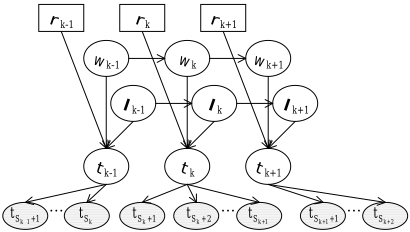
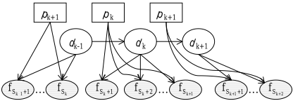
For the pitch process, the tuning is an additive offset that is added to the notated pitch to produce the observed frequency (Equation 6). In addition, we allow the frequency to deviate independent of the tuning, so Equation 6 includes a Gaussian noise term ❯ ☛ ☞ . The noise terms in Equations 4 and 6 model observational errors as well as local deviations.
Stealing:
Tuning:
Frequency: ✡
We assume that ✍ ✚ is ✜ ✘ ❉ ✙ ✢ ✎ ✛ , ✓ ✚ is ✜ ✘ ☎ ✙ ✢ ✁ ✛ , ✖ ✚ is ✜ ✘ ☎ ✙ ✢ ✗ ✛ , ❯ ✎ ❑ is ✜ ✘ ☎ ✙ ✦ ✎ ✛ , ❯ ✁ ❑ is ✜ ✘ ☎ ✙ ✦ ✁ ✛ , ❯ ❱ ❑ is ✜ ✘ ☎ ✙ ✦ ❱ ✛ , ❯ ✗ ❑ is ✜ ✘ ☎ ✙ ✦ ✗ ✛ and ❯ ☛ ☞ is ✜ ✘ ☎ ✙ ✦ ☛ ✛ , all independent of each other. The variance values used in the experiments were: ✢ ✎ ✣ ❉ ☎ ◗ ✩ , ✢ ✁ ✣ ❉ ☎ ◗ ✫ , ✢ ✗ ✣ ❉ ☎ ◗ ✁ , ✦ ✎ ✣ ❉ ☎ ◗ ✭ , ✦ ✁ ✣ ❉ ☎ ◗ ✫ , ✦ ❱ ✣ ❉ ☎ ◗ ✩ , ✦ ✗ ✣ ❉ ☎ ◗ ✩ and ✦ ☛ ✣ ❉ ☎ ◗ ✁ .
Note that we don't observe ✕ ✑ directly, but only through the durations ✟ ✝ of the individual sound events, where ✕ ✑ ✣ a80 ■ ❑ ✮ ✮ ✝ ❙ ✁ ✯ ■ ❑ ✟ ✝ . On the other hand, the model directly specifies the observed frequency ✡ ✝ of the individual sound events.
We define the rhythm prior ✷ ✘ ✓ ✁ ✙ ✆ ✆ ✆ ✙ ✓ ✍ ✛ by a Hidden Markov Model (HMM), learned offline using rhythm sequences of a corpus of music in the same style as our evaluation data. For the pitch prior we use an ❇ -grammodel (with ❇ =3), which assumes that each element in a sequence only depends on the previous ❇ ✄ ❉ elements. We define the prior over intervals rather than individual pitches since this allows for generalization to different keys. The probabilities in the model are estimated offline by the ❇ -gram frequencies in the training data.
The segmentation prior indicates, for each observed sound event, the probability that there is truly an onset immediately after the event. To obtain the segmentation prior, we use the dissimilarity values returned by the onset detector at each observation. The goal is to individually estimate ✷ ✘ onset ✝ ✺ ✲ ✝ ✛ , the probability that there is an actual onset right after the ❇ th observation, given its dissimilarity ✲ ✝ to the following observation. Although not a formal density estimation method, sigmoid fitting provides an appropriate solution [Platt, 1999]. This was suggested to transform a classifier's output values into probabilities. Using a training corpus for onset detection, we learned the following function: ✡ ✘ ✲ ✛ ✣ ✘ ❉ ❋ ✳ ✎ ✷ ✘ ✄ ✞ ✆ ✶ ✷ ✲ ❋ ✞ ✆ ✠ ✹ ✛ ✛ ◗ ✁ . The shape of the function makes sense: as the dissimilarity increases, it assigns increasing probabilities in [0,1] to the presence of an onset. In order to avoid probabilities close to 0 and 1, we used a weighted average of ✡ ✘ ✲ ✛ and ☎ ✆ ✠ as our prior: ✷ ✘ onset ✝ ✺ ✲ ✝ ✛ ✣ ☎ ✆ ✺ ✡ ✘ ✲ ✝ ✛ ❋ ☎ ✆ ✞ ✻ ☎ ✆ ✠ .
Once individual segmentation priors of all observations are computed, the prior probability of a segmentation ☞ ✁ ✄ ✍ is computed by multiplying these together:
4 Inference
Our goal is to compute the maximum a posteriori (MAP) segmentation-score configuration as given in Equation 1. Let ❄ be the set of possible note durations and ❅ the set of possible pitches. For a given observation sequence a0 ✁ ✄ ✆ , there are ✞ ✆ ◗ ✁ possible segmentations and ✘ ✺ ❄ ✺ ✻ ✺ ❅ ✺ ✛ ✍ possible scores for each segmentation with ✗ note events. The exponential number of the possible ✘ ☞ ✁ ✄ ✍ ✙ ✎ ✁ ✄ ✍ ✛ pairs makes exact computation of the MAP configuration intractable. We therefore use MCMC methods [Gilks et al., 1996] to sample from the space of possible pairs.
Our inference procedure is similar to the handling of reference uncertainty in first-order probabilistic models [Pasula and Russell, 2001]. We alternate between MCMC steps to change the segmentation, and Gibbs steps to sample the duration and pitch for a given segmentation. When changing the segmentation, reversible jump MCMC [Green, 1995] is employed since the model dimension changes whenever we split or merge events.
4.1 Reversible JumpMCMC
MCMC methods are used to generate samples from a complex target distribution where analytical or numerical techniques are not applicable. In our case, the target is the posterior distribution of the transcription given the observations, ✷ ✘ a0 ✺ a0 ✛ ✣ ✷ ✘ ☞ ✙ ✖ ✙ ✔ ✺ a0 ✛ , and we are trying to find the mode a0 ✢ of this distribution. There are well-known methods to construct a Markov chain whose stationary distribution is guaranteed to be the target distribution. In the Metropolis-Hastings algorithm, the candidate samples are generated from a proposal distribution ✢ ✘ a0 ✂ ✺ a0 ✛ and are accepted with probability ☎ ✘ a0 ✙ a0 ✂ ✛ ✣ ✩ ✝ ✞ ✠ ❉ ✙ ☛ ❀ ✌ ✎ ✑ ✓ ❂ ✔ ❀ ✌ ✑ ✌ ✎ ❂ ☛ ❀ ✌ ✑ ✓ ❂ ✔ ❀ ✌ ✎ ✑ ✌ ❂ ✗ . This is not applicable when ✷ ✘ a0 ✺ a0 ✛ does not have a fixed dimensionality, such as in our problem: different segmentations may correspond to different numbers of notes, and therefore have different numbers of parameters. The reversible jump MCMC method allows us to sample from a target distribution even when the dimensionality of the model is not fixed. The acceptance probability of moving from one model to another model of different dimension is given by:
where ✜ and ✜ ✂ aremodel indicators that determine the number of notes, a0 and a0 ✂ are the parameter vectors of sizes ✜ and ✜ ✂ respectively, ✷ ✘ ✜ ✛ is the prior probabilityofmodel ✜ , and ✷ ✙ ✙ ✎ is the probability of moving frommodel ✜ to ✜ ✂ . The function ❈ ✙ ✙ ✎ ✘ a0 ✙ ✤ ✛ ✣ ✘ a0 ✂ ✙ ✤ ✂ ✛ is a mapping between the parameters of the two models. This mapping may entail random decisions to generate the parameters a0 ✂ of ✜ ✂ given the current parameters a0 of ✜ . These decisions are denoted by the variable ✤ , whose probability distribution is ✢ ✙ ✙ ✎ ✘ a0 ✙ ✤ ✛ .
Since we assume that the segmentation, rhythm and pitch priors are independent, for the first two terms of the fraction in Equation 7 we have:
The terms in the right hand side of Equation 8 are respectively given by the segmentation prior, the rhythm prior, the pitch prior and the likelihood model.
During our sampling, we allow two kinds of moves that change the model dimension: merging two neighboring notes together, or splitting a single note into two. The rhythm and pitch components are sampled using Gibbs sampling without a change in model dimension, so we don't discuss the acceptance probability for those here and instead focus on the segmentation component ☞ of a0 . We have two possible values for ✷ ✙ ✙ ✎ : it is equal to ✷ split when ✜ ✂ ✣ ✜ ❋ ❉ and to ✷ merge when ✜ ✂ ✣ ✜ ✄ ❉ . The two functions ❈ merge and ❈ split define the mappings between the models before and after, where the move is a merge and a split respectively:
In Equation 10, because we choose the splitting point randomly from all possible boundaries between the observations currently assigned to a note, ✤ is a random variable with uniform density ✢ split ✘ ☞ ✙ ✤ ✛ ✣ ✁ ✭ ◗ ✁ . Since merging is a deterministic move, we don't have a random variable in Equation 9 so we simply have ✢ merge ✘ ☞ ✙ ✤ ✛ ✣ ❉ . Finally, it's easy to see from Equations 9 and 10 that both ✧ ✧ ✧ ✲ ✿ merge ❀ ✌ ✲ ✳ ❂ ✲ ✌ ✲ ✳ ✧ ✧ ✧ and ✧ ✧ ✧ ✲ ✿ split ❀ ✌ ✲ ✳ ❂ ✲ ✌ ✲ ✳ ✧ ✧ ✧ are equal to 1.
Putting everything together, we have the following two acceptance probabilities for merge and split moves:
where ☞ ✑ is either the total number of observations associated with the two notes we are merging, or it is the number of observations associated with the note we are splitting.
4.2 Generating Samples
Given a sample ✶ ✣ ✘ ☞ ❀ ❘ ❂ ✁ ✄ ✍ ✙ ✎ ❀ ❘ ❂ ✁ ✄ ✍ ✛ , new samples are generated as follows:
- Pick an index ✕ .
- Resample the ✕ th note, keeping the segmentation and all other notes the same:
Let a0 ✣ ✘ ☞ ❀ ❘ ✯ ✁ ❂ ✁ ✄ ✍ ✙ ✎ ❀ ❘ ✯ ✁ ❂ ✁ ✄ ✍ ✛ . It is accepted automatically as a sample since it was generated by Gibbs sampling.
- With probability ✷ merge, merge the ✕ th note with its suc-
- Change segmentation in one of two ways: cessor:
b. With probability ✷ split ✣ ❉ ✄ ✷ merge, split the ✕ th note into two at ❇ , an integer chosen uniformly at random from ✽ ❉ ✙ ☞ ✑ ✄ ❉ ❁ (only possible if ☞ ✑ ✑ ❉ ).
✗ ✂ ✸ ✗ ❋ ❉ ☞ ❀ ❘ ✯ ✩ ❂ ✑ ✸ ❇ ☞ ❀ ❘ ✯ ✩ ❂ ✑ ✯ ✁ ✸ ☞ ❀ ❘ ❂ ✑ ✄ ❇ ❃ ☞ ❀ ❘ ✯ ✩ ❂ ✷ ✙ ✎ ❀ ❘ ✯ ✩ ❂ ✷ ❄ ✸ ❃ ☞ ❀ ❘ ❂ ✷ ✙ ✎ ❀ ❘ ❂ ✷ ❄ ✙ ✹ ✻ ✽ ❉ ✿ ✕ ✄ ❉ ❁ ❃ ☞ ❀ ❘ ✯ ✩ ❂ ✷ ✙ ✎ ❀ ❘ ✯ ✩ ❂ ✷ ❄ ✸ ❃ ☞ ❀ ❘ ❂ ✷ ◗ ✁ ✙ ✎ ❀ ❘ ❂ ✷ ◗ ✁ ❄ ✙ ✹ ✻ ✽ ✕ ❋ ✞ ✿ ✗ ✂ ❁ Jointly sample values for ✎ ❀ ❘ ✯ ✩ ❂ ✑ and ✎ ❀ ❘ ✯ ✩ ❂ ✑ ✯ ✁ from ✷ ✘ ✎ ✑ ✙ ✎ ✑ ✯ ✁ ✺ ☞ ✁ ✄ ✍ ✙ ✎ ◗ ❀ ✑ ✄ ✑ ✯ ✁ ❂ ✙ a0 ✁ ✄ ✆ ✛ .
- Let a0 ✂ ✣ ✘ ☞ ❀ ❘ ✯ ✩ ❂ ✁ ✄ ✍ ✎ ✙ ✎ ❀ ❘ ✯ ✩ ❂ ✁ ✄ ✍ ✎ ✛ . It is a candidate sample that has a different segmentation than a0 . The acceptance probability of a0 ✂ as the next sample is given by one of Equations 11 and 12, decided by whether it corresponds to a merge or a split move.
In step 1 above, although we could pick a random ✕ , processing the events sequentially (✕ ✣ ❉ ✙ ✆ ✆ ✆ ✙ ✗ ) allows computational savings. We can factorize the likelihood as:
where ☎ denotes the hidden variables ✍ , ✓ , and ✖ . The first factor is computed incrementally as new samples are taken for ✕ ✣ ❉ to ✗ . The second factor depends only on the future observations, and can be efficiently computed in advance for all ✕ s by a backward filtering pass.
Given ✘ ☞ ✁ ✄ ✍ ✙ ✎ ✁ ✄ ✍ ✛ , the relationships between the continuous variables of our model are linear, and the additive change or noise variables are all Gaussian. So, it is a linear dynamical system where the integration over the hidden variables (in Equation 13) can be computed analytically using Kalman filtering. All the necessary probabilities can be represented by Gaussian potentials, over which multiplication, conditioning and marginalization are three basic operations.
A problem with this individual sampling of ✎ ✑ s is that sometimes the neighboring notes will be such that it is very unlikely to sample a good value for either one with the current assignment of the other. To overcome such deadlocks, we randomly sample some score pairs ✘ ✎ ✑ ✙ ✎ ✑ ✯ ✁ ✛ jointly in Step 2. Steps 3 and 4 are not performed for joint samples. Ideally, one would like to sample all events jointly given a segmentation, but this would result in an exponential sampling space.
We define an MCMC iteration as one sequence of samplings from ✕ ✣ ❉ to ✗ . After some iterations, we randomly propose a global sampling step. We have two global operations: one that shifts all the pitches in the sample by ✞ ❉ , and one that halves or doubles all durations. If the result of halving produces a duration not in ❄ , we randomly select the closest element in ❄ ✟ ❃ ☎ ❄ . When a zero duration is assigned to an observation, it is grouped with one of its neighbors. In the experiments we used 20 chains with 250 iterations per chain. Each chain starts with an initial sample that is obtained by matching the observations as closely as possible: If the segmentation prior of an observation is less than 0.5, we group it with its successor. The durations are rounded to the closest duration in ❄ , and the frequencies are rounded to the closest pitch in ❅ . Starting with this sample, as opposed to a random one, allows us to get to a good transcription faster.
5 Experiments
5.1 Training and Evaluation Data
A corpus of monophonic vocal music was used to evaluate the system and its various components. The corpus consisted of two parts. One part contained both scores and audio data, and was used to evaluate the system. The test data had a total duration of 60 minutes, composed of 55 audio segments containing a total of 3606 notes. All pieces were by the Renaissance composer G.P. Palestrina (16th century), and sung by the same singer. The second part of the corpus consisted only of scores without audio data. This part was used to learn the rhythm and pitch priors. There were 78 pieces by Palestrina in this part, none of which appeared in the first part. Two audio fragments were removed from the first part for the purpose of tuning the eight variance parameters of the graphical model and the two sigmoid parameters of the segmentation prior. These were not used in the evaluation.
5.2 Evaluation Metric
Given the true score ✎ ✡ ✁ ✄ ✍ ☞ and segmentation ☞ ✡ ✁ ✄ ✍ ☞ for observations a0 ✁ ✄ ✆ , we evaluate the system's result ✎ ✢ ✁ ✄ ✍ and ☞ ✢ ✁ ✄ ✍ as follows:
Segmentation: We count the number of correct onset/noonset decisions over the number of possible segmentation locations ( ✖ ✄ ❉ ).
Musical Score: Since the system's segmentation might be different from the reference segmentation, comparing ✎ ✢ ✁ ✄ ✍ directly to ✎ ✡ ✁ ✄ ✍ ☞ is not very meaningful. We instead evaluate the score by looking at the number of rhythm and pitch errors remaining once the segmentation errors are fixed. For instance if a half note is transcribed as two successive quarter notes of the same pitch, we consider this to be a segmentation error (extra onset), and not a rhythm transcription error. Similarly, if two successive quarter notes of the same pitch are transcribed as a half note, this is only a segmentation error (missed onset). If, on the other hand, two successive quarter notes of different pitches are transcribed as a half note, there is a pitch error in addition to the segmentation error. This is because even after correcting the missed onset by splitting the half note in two, our transcription would have a pitch different from the real score.
Returning to the extra onset case, if a half note is transcribed as two separate quarter notes of different pitches, then when the segmentation error is corrected the two quarter notes are replaced by a half note with a single pitch. We need to choose one of the pitches of the two quarter notes as the pitch of the half note. There may or may not be a pitch error in addition to the segmentation error, depending on which pitch is chosen for the half note. We choose to go with the pitch whose related observation is longer in duration. If this is equal to the real pitch, there is no pitch error. This generalizes naturally to cases where a single true note is transcribed as multiple notes.
For the evaluation of durations, if a note is transcribed as multiple notes (extra onsets), we compare the sum of these durations to the reference duration. If multiple notes are transcribed as a single note (missed onset), we compare the duration of this note to the sum of the reference durations. We can extend this idea to evaluate cases of misplaced onsets, where the computed transcription contains an onset in a different place from the reference transcription. In both the reference and computed transcriptions, we only keep the onsets that appear in both, and compute durations for these new segments by summing the durations of their constituents. These are then compared to evaluate the rhythm transcription.
5.3 Results
We present the results for the evaluation of our system in Tables 1 and 2. Table 1 contains the results obtained by the sampling process described in Section 4. This process generates samples from the posterior distribution of the transcription.
| Seg. | Pitch | Dur. | Comb. | Time | |
|---|---|---|---|---|---|
| All | 87.28 | 86.11 | 85.42 | 86.26 | 82.25 |
| All-R | 87.63 | 95.08 | 49.81 | 71.42 | 25.60 |
| All-P | 86.85 | 86.67 | 86.29 | 86.60 | 75.44 |
| All-SG | 83.30 | 87.01 | 82.65 | 84.28 | 82.88 |
| All-ST | 86.98 | 83.21 | 85.36 | 85.16 | 67.48 |
| All-J | 86.11 | 81.52 | 79.14 | 82.16 | 99.67 |
| None | 71.27 | 93.81 | 36.60 | 57.68 | 9.10 |
| All-RG | 65.19 | 92.38 | 62.09 | 70.97 | 71.17 |
| None-RG | 62.15 | 92.27 | 19.61 | 38.50 | 4.93 |
| Seg. | Pitch | Dur. | Comb. | Time | |
|---|---|---|---|---|---|
| All | 87.08 | 89.60 | 87.15 | 87.93 | 81.02 |
| All-R | 89.32 | 93.76 | 50.06 | 71.71 | 32.44 |
| All-P | 87.53 | 88.27 | 87.68 | 87.83 | 69.55 |
| All-SG | 83.08 | 87.15 | 83.16 | 84.42 | 82.17 |
| All-ST | 86.98 | 88.22 | 87.47 | 87.55 | 66.82 |
| All-J | 85.24 | 84.36 | 80.26 | 83.23 | 99.93 |
| None | 75.69 | 91.56 | 46.12 | 65.48 | 8.85 |
| All-RG | 65.19 | 92.38 | 62.09 | 70.97 | 71.17 |
| None-RG | 62.15 | 92.27 | 19.61 | 38.50 | 4.93 |
However, we are mainly interested in the mode of this distribution, so we do not really need to ensure that our sampling has the posterior as its stationary distribution. We could employ any search process over the space of transcriptions, and output the one with the highest posterior. Since we know that our input is over-segmented, a simple modification is to bias our sampler towards merging segments. We implement this by removing the ✘ ☞ ✑ ✄ ❉ ✛ ◗ ✁ factors from Equations 11 and 12. Other approaches such as simulated annealing can also be used to generate samples concentrated around the modes. However, we were able to obtain slightly higher posteriors with the same number of iterations using this simpler modification. The results using the modification are presented in Table 2, and we use that table to discuss our results. It is important to keep in mind that both Tables 1 and 2 use samples to approximate the MAP transcription. It is likely that the exact MAP configurations would have higher posteriors, with possibly higher or lower evaluation scores. However, given the high number of iterations, the values are still representative of the performance of their respective models.
In both Tables 1 and 2, the first three columns contain the success rates for the segmentation, pitch transcription and rhythm quantization, using the metric defined in Section 5.2. The next column contains the harmonic mean 1 of these three as a combined metric. The last column gives the average time per iteration (in msecs) for a 24.92 seconds input signal. The first row (All) refers to the system with all of the priors described in Section 3. The next three rows show the results when either prior is removed: rhythm (All-R), pitch (All-P), or segmentation (All-SG). We then present results where we don't include the stealing process given in Equation 3 (All- ST), and where we don't allow joint sampling (All-J). The next row contains the results when none of these five components is used (None). The final two rows (All-RG and None-RG) show the results when we don't allow regrouping of observations, so that every observation is a separate segment. This is what we would get if we did not reason about segmentation, and instead assumed that the onset detector is perfect. Notice that these two rows are the same in the two tables since the segmentation is fixed.
1 a0 ✁ ✄ ✆ ✞ ✆ ✡ ☞ ✍ ✏ ✑ ✓ ✕ ✑ ✓ ✗ ✑ ✕ ✗ ✓ ✕ is similar to F-measure for 3 numbers.
The most instructive comparison is between All and AllRG. We see that not only does All-RG do significantly worse on segmentation, which is expected, its score for duration is also much lower. It seems to be the case that errors in segmentation spill over, causing significant errors in rhythm as well. Surprisingly, however, All-RG does a little better on pitch transcription. This may be because it is not subject to missed onset errors, which as we saw earlier always results in a pitch error when two notes of different pitches are transcribed as a single note. Comparison of None and None-RG is similar. Again, the system that allows regrouping greatly outperforms the one that does not on segmentation and rhythm, but does slightly worse on pitch.
Now we consider the effect of individual components of the model. We see that the rhythm prior greatly improves the performance on duration, while slightly hurting the segmentation and pitch scores. It could be that without a rhythm prior, the segmentation prior and observed pitches have a greater effect on the segmentation, and the pitches can match the observations more closely. Overall, however, the small negative effect on pitch and segmentation is well compensated for by the improvement in duration. The pitch prior has only a very small effect. It leads to a slight improvement in pitch, and a slight degrading of the segmentation and duration scores. The segmentation prior and joint sampling lead to an improvement in all three scores. The stealing process has little effect, increasing the pitch score and slightly decreasing the other two scores. It might be more useful in other styles of music.
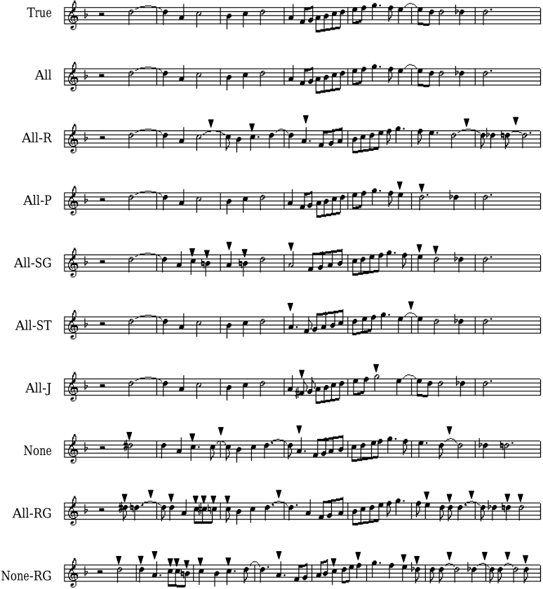
In Figure 3, we show the transcription results for a short audio segment. The true transcription is given first, followed by the transcriptions returned by each of the systems in Table 2. The errors are indicated by the arrows above them. The complete system (All) is able to transcribe the piece with no mistakes. We see that by removing the rhythm prior (All-R), we get many stylistic errors: the notated durations of the first, forth and fifth errors are very unlikely, and they induce an unlikely rhythmic pattern. Removing the segmentation prior (All-SG) results in segmentation errors, which are often accompanied by pitch and/or rhythm mistakes. We see this in the second error, where the pitch has been transcribed incorrectly once the note is split into two. The stealing prior provides flexibility to transcribe local expressive or motor deviations correctly. Without it (All-ST), we are unable to correctly transcribe the first note at the beginning of the fourth measure: its elongated performance requires a too large deviation in the global tempo to be transcribed correctly. In the bottom two rows of Figure 3, we clearly see that the two systems without reasoning about the segmentation have many mistakes, and the quality of transcription is really poor, especially for the last row. Even in the All-RG system that includes rhythm and pitch priors, we can see that segmentation errors result in many additional pitch and rhythm errors. So, we clearly see the benefits of reasoning about the segmentation in this example.
6 RelatedWork
Transcription of music signals to scores is a difficult problem. Most related work consists of addressing subproblems such as pitch tracking, onset detection, beat tracking, level 1-to2 (audio to MIDI or piano-roll), and level 2-to-3 (MIDI to score).
There are a number of related works on the level 1-to-2 problem. Most systems transform the signal into a timefrequency representation, followed by heuristic methods to segment the signal and label segments with pitch or chord names (see [Klapuri, 2004] for a more detailed literature review). Sterian (1999) proposes heuristics to pick peaks from the time-frequency image. He then uses a Kalman filter to extract partial tracks and searches over hypotheses for the association of the tracks to notes. Marolt (2004) presents a connectionist approach: oscillator networks for partial tracking and neural networks for note recognition. Raphael (2002a) computes a set of features from each frame of the timefrequency image, and takes these as observations from an HMM. Cemgil et al. (2004) propose a graphical model whose observation is directly the time domain signal.
Beat tracking is another problem related to rhythm transcription. Dixon (2001) proposes a rule-based system to estimate beats from a sequence of onset times. Goto and Muraoka (1998) take an audio signal as input and use DSP methods to construct and select frommultiple beat hypotheses. We consider beats to lie somewhere between levels 2 and 3: given perfect onset times, the beats could be used to assign discrete durations to observed events. However, onset detection accuracy is not crucial for beat trackers. On the contrary, poor onset detection seems to help beat tracking by filtering out less salient onsets. This is clearly undesirable for a transcription system.
There have been systems employing graphical models for level 2-to-3 problem: Given a list of onset times, Cemgil and Kappen (2003) use MCMC methods to sample most likely note durations. Raphael (2002b) proposes an exact method for the joint estimate of the tempo and note durations. He introduces a "thinning" operation that removes a value from consideration for a discrete variable, if that variable is guaranteed not to have that value in the MAP configuration. This seems to keep the search space from growing exponentially. However, both of these systems assume that their list of onset times is accurate, so they have a one-to-one mapping between observations and score events. In our case, the number of mappings alone is exponential, which is why we chose approximate methods.
We believe that exploiting the advances in DSP to get to level 2 (even a noisy one), and then using graphical models for level 2-to-3 is appropriate. Level 2 data is much more instrument independent, and it is much shorter. However, without perfect onset detectors in sight, level 2 data will inevitably have errors, and our experiments have shown that these errors are magnified in the subsequent analysis to get to level 3. The most important contribution of our system is its ability to accept and reason about noisy input. To the best of our knowledge, it is the first music transcription system to go from level 1 to level 3 without assuming a perfect level 2.
7 Discussion and Conclusion
We have presented a transcription system that takes a music signal as input and returns its musical score. We use a noisy onset detector as our front-end, which computes the input to a family of graphical models. Each regrouping of this input corresponds to a specific model from this family. Our inference procedure jointly searches over models and scores that may have produced the observed sound events. Our results show that this is a very well-suited approach to the problem of music transcription.
The constraint on our onset detection noise is that we can have extra onsets but not many missed onsets, since these will be reflected as merged notes in the final score. This is a reasonable requirement, as most detectors can be tuned to reduce missed onset at the cost of increased extra onsets. We can therefore use a variety of onset detectors as our frontend. Also, in theory we could apply our system to individual frames, although the inference would take much longer.
In our models, the pitch and rhythm variables are conditionally independent given the segmentation. This keeps the sampling over the two spaces separate. A more sophisticated model could combine the rhythm and pitch processes as well as the priors. Also, the rhythm and pitch priors we learn are style-specific due to the homogeneity of the training data. This makes sense, as a trained musician would transcribe the same audio signal differently under different stylistic assumptions. Ultimately, we would like to have rhythm priors for various styles and make the choice of style a variable that needs to be optimized as well.
@inproceedings{ijcai2005p61,
  title     = {Signal-to-Score Music Transcription using Graphical Models},
  author    = {Kapanci, Emir and Pfeffer, Avi},
  booktitle = {Proceedings of the Nineteenth International Joint Conference on
               Artificial Intelligence, {IJCAI-05}},
  publisher = {International Joint Conferences on Artificial Intelligence},
  editor    = {Leslie Pack Kaelbling and Alessandro Saffiotti},
  pages     = {758--764},
  year      = {2005},
  url       = {https://ijcai.org/proceedings/2005/61},
}
TY - CPAPER TI - Signal-to-Score Music Transcription using Graphical Models AU - Kapanci, Emir AU - Pfeffer, Avi T2 - Proceedings of the Nineteenth International Joint Conference on Artificial Intelligence, IJCAI-05 PB - International Joint Conferences on Artificial Intelligence PY - 2005 SP - 758 EP - 764 UR - https://ijcai.org/proceedings/2005/61 ER -Copied
Machine-readable versions of this paper, for tools and AI agents:





