
Cho-k-NN: A Method for Combining Interacting Pieces of Evidence in Case-Based Learning
Proceedings of the Nineteenth International Joint Conference on Artificial Intelligence. Pages 3-7.
© 2005 International Joint Conferences on Artificial Intelligence
Abstract
The case-based learning paradigm relies upon memorizing cases in the form of successful problem solving experience, such as e.g. a pattern along with its classification in pattern recognition or a problem along with a solution in case-based reasoning. When it comes to solving a new problem, each of these cases serves as an individual piece of evidence that gives an indication of the solution to that problem. In this paper, we elaborate on issues concerning the proper combination (aggregation) of such pieces of evidence. Particularly, we argue that cases retrieved from a case library must not be considered as independent information sources, as implicitly done by most case-based learning methods. Focusing on the problem of prediction as a performance task, we propose a new inference principle that combines potentially interacting pieces of evidence by means of the so-called (discrete) Choquet-integral. Our method, called Cho-k-NN, takes interdependencies between the stored cases into account and can be seen as a generalization of weighted nearest neighbor estimation.
- [Aha et al., 1991] D.W. Aha, D. Kibler, and M.K. Albert. Instance-based learning algorithms. Machine Learning, 6(1):37-66, 1991.
- [Aha, 1997] D.W. Aha, editor. Lazy Learning. Kluwer Aca- demic Publ., 1997.
- [Choquet, 1954] G. Choquet. Theory of capacities. Annales de l'Institut Fourier, 5:131-295, 1954.
- [Dasarathy, 1991] B.V. Dasarathy, editor. Nearest Neighbor (NN) Norms: NN Pattern Classification Techniques. IEEE Computer Society Press, Los Alamitos, California, 1991.
- [Dudani, 1976] S.A. Dudani. The distance-weighted k- nearest-neighbor rule. IEEE Transactions on Systems, Man, and Cybernetics, SMC-6(4):325-327, 1976.
- [Grabisch, 1997] M. Grabisch. k-order additive discrete fuzzy measures and their representation. Fuzzy Sets and Systems, 92:167-189, 1997.
- [Hüllermeier, 2002] E. Hüllermeier. On the representation and combination of evidence in instance-based learning. In Proc. ECAI-2002, pages 360-364, Lyon, France, 2002.
- [Hume, 1999] D. Hume. An Enquiry concerning Human Un- derstanding. Oxford Univ. Press Inc., New York, 1999.
- [Kolodner, 1993] J.L. Kolodner. Case-based Reasoning. Morgan Kaufmann, San Mateo, 1993.
- [Lindenbaum et al., 1999] M. Lindenbaum, S. Marcovich, and D. Rusakov. Selective sampling for nearest neighbor classifiers. AAAI-99, pages 366-371, Orlando, 1999.
- [McSherry, 2002] D. McSherry. Diversity-concious re- trieval. ECCBR-02, pages 219-233. Springer, 2002.
- [Murofushi and Soneda, 1993] T. Murofushi and S. Soneda. Techniques for reading fuzzy measures (iii): interaction index. In 9th Fuzzy System Symposium, pages 693-696.
- [Oliver and Webster, 1990] M. Oliver, R. Webster. Kriging: a method of interpolation for geographical information system. Int. J. Geogr. Inform. Syst., 4(3):313-332, 1990.
- [Rendell, 1986] L. Rendell. A general framework for induc- tion and a study of selective induction. Machine Learning, 1:177-226, 1986.
- [Riesbeck and Schank, 1989] C.K. Riesbeck and R.C. Schank. Inside Case-based Reasoning. Hillsdale, New York, 1989.
- [Schapire et al., 1998] RE. Schapire, Y. Freund, P. Bartlett, and WS. Lee. Boosting the margin: a new explanation for the evectiveness of voting methods. Annals of Statistics, 26:1651-1686, 1998.
- [Sugeno, 1974] M. Sugeno. Theory of Fuzzy Integrals and its Application. PhD thesis, Tokyo Inst. of Techn., 1974.
- [Wettschereck et al., 1997] D. Wettschereck, D.W. Aha, and T. Mohri. A review and empirical comparison of feature weighting methods for a class of lazy learning algorithms. AI Review, 11:273-314, 1997.
- [Zhang et al., 1997] J. Zhang, Y. Yim, and J. Yang. Intelli- gent selection of instances for prediction in lazy learning algorithms. Art. Intell. Review, 11:175-191, 1997.
References were extracted automatically from the PDF and may contain errors.
Full text extracted automatically from the PDF; figures, tables and equations may differ. The PDF is the version of record.
1 Introduction
Case-based or instance-based learning algorithms have been applied successfully in �elds such as, e.g., machine learning and pattern recognition during the recent years [Aha et al., 1991; Dasarathy, 1991]. The case-based learning (CBL) paradigm is also of central importance in case-based reasoning (CBR), a problem solving methodology which goes beyond the standard prediction problems of classi�cation and regression [Riesbeck and Schank, 1989; Kolodner, 1993].
As the term suggests, in CBL special importance is attached to the concept of a case. A case or an instance can be thought of as a single experience, such as a pattern (along with its classi�cation) in pattern recognition or a problem (along with a solution) in CBR.
Rather than inducing a global model (theory) from the data and using this model for further reasoning, as inductive, model-based machine learning methods typically do, CBL systems simply store the data itself. The processing of the data is deferred until a prediction (or some other type of query) is actually requested, a property which quali�es CBL as a lazy learning method [Aha, 1997]. Predictions are then derived by combining the information provided by the stored cases, primarily by those which are similar to the new query.
In fact, the concept of similarity plays a central role in CBL. The major assumption underlying CBL has already been expressed, amongst others, by the philosopher DAVID HUME ([Hume, 1999], page 116): �In reality, all arguments from experience are founded on the similarity ... among natural objects. ... From causes, which appear similar, we expect similar effects.� This commonsense principle, that we shall occasionally call the �similarity hypothesis� [Rendell, 1986], serves as a basic inference paradigm in various domains of application. For example, in a classi�cation context, it translates into the assertion that �similar objects have similar class labels�, and in CBR it suggests that �similar problems have similar solutions�.
The similarity hypothesis, which is apparently of a heuristic nature, has been put into practice by means of different inference schemes that combine similarity and frequency information in one way or the other. For example, the well-known nearest neighbor (NN) classi�er �rst selects a neighborhood around the query, consisting of the k most similar cases, and then counts the occurrence of the different class labels. Despite of their simplicity, inference methods of such kind have proved to be quite successful in practical applications.
In this paper, we suggest a further improvement based on the idea of taking interdependencies between neighbored cases into account. In fact, in standard NN methods, these cases are implicitly considered as independent information sources. We argue that a corresponding assumption of independence is not always justi�ed and propose a new inference principle that combines interacting pieces of evidence in a more thorough way. This principle, which makes use of non-additive measures for modeling interaction between cases and employs the so-called (discrete) Choquet-integral as an aggregation operator, can be seen as a generalization of weighted NN estimation.
By way of background, section 2 gives a concise review of the NN principle, which constitutes the core of the family of CBL algorithms. In section 3, we discuss the problem of interaction between cases in CBL. A new approach to CBL, which takes such interactions into account, is then introduced in section 4 and evaluated empirically in section 5.
2 Nearest Neighbor Estimation
The well-known nearest neighbor (NN) estimation principle is applicable to both classi�cation problems (prediction of class labels) and regression (prediction of numeric values).
Consider a setting in which an instance space X is endowed with a similarity measure sim : X × X → [0, 1]. An instance corresponds to the description x of an object (usually in attribute�value form). In the standard classi�cation framework, each instance x is assumed to have a (unique) label y ∈ L. Here, L is a �nite (typically small) set comprised of m class labels {ℓ1 . . . ℓm}, and 〈x, y〉 ∈ X ×L is a labeled instance (case).
The NN principle originated in the �eld of pattern recognition [Dasarathy, 1991]. Given a sample S consisting of n labeled instances 〈xı, yı〉, 1 ≤ ı ≤ n, and a novel instance x0 ∈ X (a query), this principle prescribes to estimate the label y0 of the yet unclassi�ed query x0 by the label of the nearest (most similar) sample instance. The k-nearest neighbor (k-NN) approach is a slight generalization, which takes the k ≥ 1 nearest neighbors of x0 into account. That is, an estimation yest 0 of y0 is derived from the set Nk(x0) of the k nearest neighbors of x0, usually by means of a majority vote. Besides, further conceptual extensions of the (k-)NN principle have been devised, such as distance weighting [Dudani, 1976]:
where ωx is the weight of the instance x and I(·) the standard {true, false} → {0, 1} mapping. (Throughout the paper, we assume the weights to be given by ωx = sim(x, x0).)
The NN principle can also be used for regression problems, i.e., for realizing a (locally weighted) approximation of realvalued target functions x ↦→ y = f(x) (in this case, L = R). To this end, one reasonably computes the (weighted) mean of the k nearest neighbors of a new query point:
3 Interaction Between Cases in CBL
Some case-based approaches completely rely on the (supposedly) most relevant piece of evidence, namely the observation which is most similar to the query. In CBR, for example, it is common practice to retrieve just a single case from the case library, and to adapt the corresponding solution to the problem under consideration. On the one hand, ignoring all but the most similar observation is conceptually simple and computationally ef�cient. On the other hand, this approach does of course come along with a loss of information, because only a very small part of the past experience is utilized.
If several instead of only a single case are retrieved, as e.g. in k-NN, an important question arises: How should the pieces of evidence coming from the different cases be combined? In k-NN classi�cation, the evidences in favor of a certain class label are simply added up (see (1)). Likewise, in regression the estimation is a simple linear combination of the observed outcomes (see (2)). Thus, the neighbored cases are basically considered as independent information sources.
This assumption of independence between case-based evidence can thoroughly be called into question [H¤ullermeier, 2002]. Indeed, it is not even in agreement with the similarity hypothesis itself! Namely, if this hypothesis is true, then two neighbored cases that are not only similar to the query case but also similar among each other will probably provide similar information regarding the query. In other words, when taking the similarity hypothesis for granted, the information coming from the neighbored cases is at least not independent.
In particular, from a problem solving perspective, one should realize that a set of cases can be complementary in the sense that the experiences represented by the individual cases complement or reinforce each other. On the other hand, cases can also be redundant in the sense that much of the information is already represented by a smaller subset among them. And indeed, as we said before, the similarity hypothesis suggests that similar cases are likely to be redundant.
To illustrate this point by a simple example, consider the problem of predicting student Peter's grade in computer science, knowing that he has an A in French. The latter information (i.e. the case 〈French,A〉) clearly suggests that Peter is an excellent student and, hence, supports predicting an A or maybe a B. Yet, one cannot be sure that this prediction is correct. In this situation, the additional information that Peter has a B in mathematics is probably more valuable than the information that he has an A in Spanish as well. In fact, the cases 〈French, A〉 and 〈Spanish, A〉 are partly redundant, since the two subjects are quite similar by themselves. As opposed to this, the case 〈mathematics, B〉 is complementary in a sense, as it suggests that Peter is not only good in languages.
Now, suppose that you know all three grades (mathematics, Spanish, French). Is A or B the more likely grade? Of course, mathematics is more similar to computer science than Spanish and French. However, depending on the concrete speci�cation of similarity degrees between the various subjects, it is quite possible that the weighted k-NN rule favors grade A since the two moderately similar A's compensate for the more similar B. Of course, this result might be judged critically, and one might wonder whether the grade A should really count twice. In fact, one reasonable alternative is to consider the two A's as only a single piece of evidence, telling something about Peter's achievements in languages, instead of two pieces of distinct information. In any case, the close connection between the two A's should not be ignored when combining the three observations.
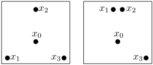
As a second example, consider the problem of predicting the yearly rainfall at a certain location (city). For instance, given the rainfall yı at location xı (ı = 1, 2, 3), what about the rainfall at location x0 in the two scenarios shown in Fig. 1? The important point to notice is that even though the individual distances between x0 and the xı are the same in both scenarios, the yı should not be combined in the same way. In this example, this is due to the different arrangements of the neighbors [Zhang et al., 1997]: Simply predicting the arithmetic mean (y1 + y2 + y3)/3 seems to be reasonable in the left scenario, while the same prediction appears questionable in the scenario shown in the right picture. In fact, since x1 and x2 are closely neighbored in the latter case, information about the rainfall at these locations will be partly redundant. Consequently, the weight of the (joint) evidence that comes from the observations 〈x1, y1〉 and 〈x2, y2〉 should not be twice as high as the weight of the evidence that comes from 〈x3, y3〉.
The above examples show the need for taking interdependencies between observed cases into account and, hence, provide a motivation for the method that will be proposed in the following section. Before proceeding, let us make two further remarks: First, the above type of interaction between cases seems to be less important if the sample size is large and even becomes negligible in asymptotic analyses of NN principles. In fact, strong results on the performance of NN estimation can be derived [Dasarathy, 1991], but these are valid only under idealized statistical assumptions and arbitrarily large sample sizes. Roughly speaking, if the sample size n tends to in�nity, the distance between the query and its nearest neighbors becomes arbitrarily small (with high probability). This holds true even if the size k of the neighborhood is increased too, as a function k(n) of n, provided that k(n)/n → 0 for n → ∞. Moreover, if the individual observations are independent and identically distributed in a statistical sense, the neighborhood becomes �well distributed�. Under these assumptions, it is intuitively clear that interdependencies between observations will hardly play any role. On the other hand, it is also clear that statistical assumptions of such kind will almost never be satis�ed in practice.
The second remark concerns related work. In fact, there are a few methods that �t into the CBL framework and that allow for taking certain types of interaction between observations into account. Particularly, these are methods that make assumptions on the statistical correlation between observations, depending on their distance [Lindenbaum et al., 1999]. For example, in our rainfall example one could employ a method called kriging, which is well-known in geostatistics [Oliver and Webster, 1990]. Usually, however, such methods are specialized on a particular type of application and, moreover, make rather restrictive assumptions on the mathematical (metric) structure of the instance space. Our approach, to be detailed in the next section, is much more general in the sense that it only requires a similarity measure sim(·) to be given. We do not make any particular assumptions on this measure (such as symmetry or any kind of transitivity), apart from the fact that it should be normalized to the range [0, 1]. From an application point of view, this seems to be an important point. In CBR, for example, cases are typically complex objects that cannot easily be embedded into a metric space.
4 The Cho-k-NNMethod
4.1 Non-Additive Measures
Let X be a �nite set and ν(·) a measure 2X → [0, 1]. For any A ⊆ X, we interpret ν(A) as the weight or, say, the degree of relevance of the set of elements A.
A standard assumption on the measure ν(·), which is made e.g. in probability theory, is additivity: ν(A ∪ B) = ν(A) + ν(B) for all A, B ⊆ X s.t. A ∩ B = ∅. Unfortunately, additive measures cannot model any kind of interaction between elements: Extending a set of elements A by a set of elements B always increases the weight ν(A) by the weight ν(B), regardless of A and B.
Suppose, for example, that the elements of two sets A and B are complementary in a certain sense. To illustrate, one might think of X as a set of workers in a factory, and of a weight ν(A) as the productivity of a team of workers A. In that case, complementarity means that the output produced by two teams A and B is higher if they cooperate. Formally, this can be expressed as a positive interaction: ν(A ∪ B) > ν(A) + ν(B). Likewise, elements can interact in a negative way. For example, if two sets A and B are partly redundant or competitive, then ν(A ∪ B) < ν(A) + ν(B).
The above considerations motivate the use of non-additive measures, also called fuzzy measures, which are simply normalized and monotone [Sugeno, 1974]:
- ν(∅) = 0, ν(X) = 1
- ν(A) ≤ ν(B) for A ⊆B
In order to quantify the interaction between subsets of a set X, as induced by a fuzzy measure ν(·), several indices have been proposed in the literature. For two individual elements xı, x ∈ X, the interaction index is de�ned by
where |A| denotes the cardinality of A and
The latter can be seen as the marginal interaction between xı and x in the context A [Murofushi and Soneda, 1993]. The above index can be extended from pairs xı, x to any set U ⊆ X of elements [Grabisch, 1997]:
where
4.2 Modeling Interaction in Case-Based Learning
Now, recall our actual problem of combining evidence in case-based learning. In this context, the set X of elements corresponds to the neighbors of the query case x0:
Our comments so far have shown that fuzzy measures can principally be used for modeling interaction between cases. The basic question that we have to address in this connection is the following: What is the evidence weight or simply the weight, ν(A), of a subset A of the neighborhood (3)?
First, the boundary conditions ν(∅) = 0 and ν(X) = 1 should of course be satis�ed, expressing that the full evidence is provided by the complete neighborhood X. Moreover, according to our comments on the similarity hypothesis (section 3), the evidence coming from a set of cases A ⊆ X should be discounted if these cases are similar among themselves. Likewise, the weight of A should be increased if the cases are �diverse� (hence complementary) in a certain sense. 1 To express this idea in a more rigorous way, we de�ne the diversity of a set of cases A by the average pairwise dissimilarity:
(By de�nition, the diversity is 0 for singletons and the empty set.) We furthermore de�ne the relative diversity by
Now, the idea is to modify the basic (additive) measure
where c = ∑xı∈X sim(x0, xı), by taking the diversity of A into account. Of course, this can be done in different ways. Here, we used the following approach:
As can be seen, the original measure µ(A) of a set of cases A is increased if the diversity of A is relatively high, otherwise it is decreased. The parameter α ≥ 0 controls the extent to which interactions between cases are taken into consideration: µ(A) can be modi�ed by at most (100 α)%. For α = 0, interactions are completely ignored and the original measure µ(·) is recovered.
For the measure ¯ ν(·) as de�ned in (5), the monotonicity condition does not necessarily hold. To remedy this problem, we simply enforce this property by setting
Finally, the boundary conditions are guaranteed by dividing the measure thus obtained by ν(X).
To illustrate, consider again the rainfall example in the right picture of Fig. 1 and suppose that sim(xı, x0) = .5 (ı = 1, 2, 3), sim(x1, x2) = .9, sim(x1, x3) = sim(x2, x3) = 0, With α = 1/2 in (5), we obtain the following weights:
1 The idea of �diversity� of a set of cases plays also a role in case-based retrieval [McSherry, 2002]. Here, however, the problem is more to �nd diverse cases, rather than to combine them.
As can be seen, the joint weight of {x1, x2} is relatively low, re�ecting the partial redundance of the two cases.
Before going on, let us comment on the derivation of the measure ν(·) from the similarity function sim(·). Firstly, even though the measure (6) captures our intuitive idea of decreasing (increasing) the evidence weight of cases that are (dis)similar by themselves, we admit that it remains ad hoc to some extent, and by no means we exclude the existence of better alternatives. For example, an interesting idea is to derive the measure in an indirect way: First, the interaction indices Iν(·) from section 4.1 are de�ned, again based on the similarity between cases. These indices can be seen as constraints on the measure ν(·), and the idea is to �nd a measure that is maximally consistent with these constraints.
Secondly, even though the assumption that similar cases provide redundant information is supported by the similarity hypothesis, one might of course argue that the similarity between the predictive parts of two cases, xı and x, is not suf�cient to call them redundant. Rather, the associated output values yı and y should be similar as well. Indeed, if y1 differs drastically from y2, the �rst two measurements in our rainfall example might better be considered as non-redundant. (In that case, the two measurements in conjunction suggest that there is something amiss ...) This conception of redundancy can easily be represented by deriving ν(·) from an extended similarity measure sim′ (·) which is de�ned over X × L. 2
Anyway, the important point of this section is not so much the speci�cation of a particular evidence measure, but rather the insight that non-additive measures can in principle be used for modeling the interaction between cases in CBL.
4.3 Aggregation of Interacting Pieces of Evidence
So far, we have a tool for modeling the interaction between different pieces of evidence in case-based learning. The next question that we have to address is how to combine these pieces of evidence, i.e., how to aggregate them in agreement with the evidence measure ν(·).
For the time being we focus on the problem of regression. Recall that in the standard approach to NN estimation, an aggregation of the output values f(xı) = yı is realized by means of a simple weighted average:
where µ({xı}) = sim(x0, xı) (∑xı∈X sim(x0, xı))-1 . Interestingly, (7) is nothing else than the standard Lebesgue integral of the function f : X →Rwith respect to the additive measure (4):
In order to generalize this estimation, an integral with respect to the non-additive measure ν(·) is needed: the Choquet integral, a concept that originated in capacity theory [Choquet, 1954].
2 We didn't explore this alternative in detail so far.
Let ν(·) be a fuzzy measure and f(·) a non-negative function. 3 The Choquet integral of f(·) with respect to ν(·) is then de�ned by
where [f > t] = {x | f(x) > t}. The integral on the righthand side is the standard Lebesgue integral (with respect to the Borel measure on [0, ∞)). In our case, where X is a �nite set, we can refer to the discrete Choquet integral which can be expressed in a rather simple form:
where π(·) is a permutation of {1 . . . k} such that 0 ≤ f(xπ(1)) ≤ . . . ≤ f(xπ(k)), and Aı = {xπ(1) . . . xπ(ı)}.
The discrete Choquet integral (8) can be seen as a special type of aggregation operator, namely a generalized arithmetic mean. Indeed, (8) coincides with (7) if ν(·) is an additive measure (i.e. if ν(·) = µ(·)). Otherwise, it is a proper generalization of the standard (weighted) NN estimation.
Coming back to our running example, suppose that we have measured the following rainfalls: y1 = 100, y2 = 120, y3 = 200. According to (8), we then obtain the estimation yest 0 ≈ 157. As the joint weight of the two locations with less rainfall, x1 and x2, has been decreased, this estimation is higher (closer to y3) than the standard weighted NN estimation given by yest 0 = 140.
So far, we have focused on the problem of regression. In the case of classi�cation, the Choquet integral cannot be applied immediately, since an averaging of class labels yı does not make sense. Instead, the Choquet integral can be derived for each of the indicator functions fℓ : y ↦→ I(y = ℓ), ℓ = ℓ1 . . . ℓm. As in (1), the evidence in favor of each class label is thus accumulated separately. Now, however, the interaction between cases is taken into account. As usual, the estimation is then given by the label with the highest degree of accumulated evidence.
5 Empirical Validation
In order to validate the extension of NN estimation as proposed in the previous section, we have performed several experimental studies using benchmark data sets from the UCI repository 4 and the StatLib archive. 5
Experiments were performed in the following way: A data set is randomly split into a training and a test set of the same size. For each example in the test set, a prediction is derived using the training set in combination with weighted k-NN resp. Cho-k-NN. In the case of regression, an estimation y est 0 is evaluated by the relative estimation error |y est 0 -y0|·|y0|-1 , and the overall performance of a method by the mean of this error over all test examples. In the case of classi�cation, we simply took the misclassi�cation rate as a performance index. Moreover, we derived statistical estimations of the expected performance of a method by repeating each experiment 100 times.
3 The Choquet integral can be extended to any real-valued function through decomposition into a positive and negative part.
4 http://www.ics.uci.edu/˜mlearn
5 http://stat.cmu.edu/
| data set | k | weighted k-NN | Cho-k-NN |
|---|---|---|---|
| auto-mpg | 5 7 | 12.21(0.05) 12.18(0.06) | 11.56(0.05) 11.53(0.05) |
| bolts | 5 7 | 47.07(1.19) 51.36(1.25) | 38.77(0.71) 39.94(0.81) |
| housing | 5 7 | 14.83(0.08) 14.99(0.09) | 14.48(0.08) 14.62(0.08) |
| detroit | 5 7 | 16.02(0.55) 15.93(0.55) | 14.90(0.50) 14.71(0.54) |
| echomonths | 5 7 | 97.77(7.17) 99.03(8.98) | 72.87(3.87) 74.80(7.55) |
| pollution | 5 7 | 4.12(0.05) 4.22(0.05) | 4.05(0.05) 4.18(0.05) |
For the purpose of similarity computation, all numeric attributes have �rst been normalized to the unit interval by linear scaling. The similarity was then de�ned by 1-distance for numeric variables and by the standard 0/1-measure in the case of categorical attributes. The overall similarity sim(·) was �nally obtained by the average over all attributes. As the purpose of our study was to compare �under equal conditions � weighted k-NN with Cho-k-NN in order to verify whether or not taking interactions into account is useful, we refrained from tuning both methods, e.g. by including feature selection or feature weighting (even though it is wellknown that such techniques can greatly improve performance [Wettschereck et al., 1997]). Results have been derived for neighborhood sizes of k = 5 and k = 7; the parameter α in (5) has always been set to 1/2.
The application of Cho-k-NN for regression has shown that it consistently improves weighted k-NN, sometimes only slightly but often even considerably. Some results are shown in table 1. In particular, it seems that the smaller the size of the data set, the higher the gain in performance. This �nding is intuitively plausible, since for large data sets the neighborhoods of a query tend to be more �balanced�; as already said, the neglect of interaction is likely to be less harmful under such circumstances.
For classi�cation problems, it is also true that Cho-k-NN consistently outperforms weighted k-NN; see table 2. Usually, however, the gain in classi�cation accuracy is only small, in many cases not even statistically signi�cant. Again, this is especially true for large data sets, and all the more if the classi�cation error is already low for standard k-NN. Nevertheless, one should bear in mind that, in the case of classi�cation, the �nal prediction is largely insensitive toward modi�cations of the estimated evidences in favor of the potential labels. In fact, in this study we only checked whether the �nal prediction is correct or not and, hence, used a rather crude quality measure. More subtle improvements of an estimation such as, e.g., the enlargement of an example's margin [Schapire et al., 1998], are not honored by this measure. For the future, we therefore plan to complement our results by more sophisticated experimental comparisons.
| data set | k | weighted k-NN | Cho-k-NN |
| glass | 5 7 | 33.58(0.34) 34.54(0.37) | 33.23(0.35) 33.77(0.39) |
| wine | 5 7 | 3.52(0.20) 3.27(0.20) | 3.48(0.20) 3.25(0.20) |
| zoo | 5 7 | 10.43(0.60) 11.65(0.51) | 10.08(0.60) 11.35(0.52) |
| ecoli | 5 7 | 16.30(0.25) 16.17(0.24) | 16.29(0.24) 16.11(0.24) |
| balance | 5 7 | 15.62(0.14) 13.28(0.16) | 15.23(0.16) 13.15(0.16) |
| derma | 5 7 | 3.75(0.13) 3.57(0.12) | 3.68(0.13) 3.46(0.11) |
6 Concluding Remarks
This paper has motivated the consideration of mutual dependencies between cases that represent past experience in casebased learning. The basic idea is that a combination of two or more cases can provide complementary but also redundant evidence. In order to model this type of interaction in a formal way, we have proposed the use of non-additive measures. The aggregation of different pieces of evidence can then be accomplished by means of the Choquet integral. The inference scheme thus obtained, referred to as CHO-k-NN, is a direct extension of the standard weighted NN estimation (which is recovered in the case of an additive measure).
Our experimental results have shown that CHO-k-NN consistently outperforms standard (weighted) k-NN on publicly available benchmark data. Sometimes, only marginal improvements can be achieved, particularly in the case of classi�cation and all the more for large, �well-distributed� data sets, but for many problems CHO-k-NN is considerably better than k-NN. All things considered, it can be said that taking interaction between cases in CBL into account is worthwhile by any means (mostly it helps, at worst it remains ineffective).
As already said, the derivation of a non-additive measure ν(·) from the similarity function sim(·) as outlined in section 4 is only a �rst attempt which leaves scope for development. In particular, the degree to which a set of cases is complementary resp. redundant might not only depend on their mutual similarity but also on other aspects.
We have explained how to use the Choquet integral as an aggregation operator in both regression and classi�cation problems. An interesting question concerns the extension of our approach to more general problem solving tasks as they are typically found in case-based reasoning. Even though it is obvious that the approach cannot be transferred immediately, the basic ideas and concepts might still be useful. In any case, the concrete solution will strongly depend on the particular type of application.
@inproceedings{ijcai2005p40,
  title     = {Cho-k-NN: A Method for Combining Interacting Pieces of Evidence in Case-Based Learning},
  author    = {Hüllermeier, Eyke},
  booktitle = {Proceedings of the Nineteenth International Joint Conference on
               Artificial Intelligence, {IJCAI-05}},
  publisher = {International Joint Conferences on Artificial Intelligence},
  editor    = {Leslie Pack Kaelbling and Alessandro Saffiotti},
  pages     = {3--7},
  year      = {2005},
  url       = {https://ijcai.org/proceedings/2005/40},
}
TY - CPAPER TI - Cho-k-NN: A Method for Combining Interacting Pieces of Evidence in Case-Based Learning AU - Hüllermeier, Eyke T2 - Proceedings of the Nineteenth International Joint Conference on Artificial Intelligence, IJCAI-05 PB - International Joint Conferences on Artificial Intelligence PY - 2005 SP - 3 EP - 7 UR - https://ijcai.org/proceedings/2005/40 ER -Copied
Machine-readable versions of this paper, for tools and AI agents:





