Model minimization by linear PSR

1 Introduction

Efficient decision making under uncertainty requires ignoring irrelevant details of a complex dynamical system and focusing on useful abstractions. A traditional representation for stochastic dynamical systems is provided by Partially Observable Markov Decision Processes (POMDPs). An attractive alternative to POMDPs is the Predictive State Representation (PSR), introduced in [Littman et al., 2002] and further developed in [Singh et al., 2004]. PSRs can be used to represent a larger class of dynamical systems than POMDPs. Even for systems that can be represented as POMDPs, PSRs hold the promise of a more compact representation. In particular, Littman et al (2002) show that a PSR representation is no larger than the number of states in a POMDP. We point out a special case of their linear PSR representation, in which a strict reduction in the number of states is obtained. We believe this special case is interesting because it relies only on the state dynamics, without taking into account the observations. This can be potentially attractive, especially for robotics applications, in which states can have similar dynamics but sensor reading will often be different.

2 Preliminaries

A POMDP representation of a dynamical system includes the following components: a finite unobservable state space S; a finite action space A; a finite observation space O; a transition function T : S×A×S→R , T(s,a, s′ ) = P(st+1 = s′ |st = s, at = a); an observation function O : S×A×O →R , O(o, s, a) = P(ot+1 = o|st+1 = s, at = a); an initial belief state b0, which is a vector of size |S|, giving the initial probability of the system being in each underlying state; and a reward function R : S×A→R , where R(s,a) is the immediate expected reward. We will not be concerned here with rewards, we will consider just actions and observations.

We denote by T a an |S|×|S| matrix containing state transition probabilities for action a. We denote by O ao a diagonal

Doina Precup

McGill University School of Computer Science dprecup@cs.mcgill.ca

matrix of size |S|×|S|, in which the diagonal elements correspond to the probabilities of emitting o from each state, given that the state is reached by action a. A test is defined as an ordered sequence of action-observation pairs t = a0o1...an-1on, which can happen from the current time step into the future. The conditional probability of test t given a prior history h of action-observation pairs is p(t|h) = p(o1...on|h,a0...an-1).

A set of tests Q = {q1...qm} constitutes a linear PSR if, for any history, the probability of any other test t can be computed as a linear combination of the predictions for the tests in Q. In other words, for any test t there exists a vector mt of size |Q|, such that p(t|h) = p(Q|h)T mt ,∀h.

Littman et al. also define an outcome function u mapping tests into n-dimensional vectors defined recursively by: u(ε) = 1|S| and u(aot) = (T a O a,o u(t)) where ε represents a null test and en is the (1×n) vector of all 1s. Each component ui(t) indicates the probability of the test t when its sequence of actions is applied from state i. A set of tests Q is called linearly independent if the outcome vectors of its tests u(q1),u(q2), ...u(qm) are linearly independent.

PSRs are related to POMDPs through the state-test prediction matrix U [Littman et al., 2002]. The rows of U correspond to states in S and columns correspond to all possible tests in order of increasing length. The entry Ui j is the conditional probability of the jth test given that the state of the system is i. A linear PSR can be derived from the matrix U by searching for a maximal set of linearly independent columns of U. Following the definition of outcome function,

where t j = a0o1...an-1on. The maximum number of linearly independent columns is the rank of U. Therefore the size of Q is upper-bounded by the number of states. Next section presents a special case in which |S| is strictly greater than |Q|.

3 Linearly dependent states

We say that a state i is linearly dependent on a subset of states S′ ⊂ S if and only if its transition probabilities under any action a are a linear combination of the transition probabilities of states in S′ under the same action:

where ∑k∈S′ ck = 1 and there exists k such that ck ̸= 0. Note that the coefficients ck will be used to weigh the transitions corresponding to state k for all of the actions. Hence, these coefficients have to be shared across the actions.

Theorem: If the underlying MDP of a given POMDP has a linearly dependent states, then a linear PSR will provide a compression of the state space.

Proof: Suppose there exists a state i ∈ S which is linearly dependent on a set of states S′ , so:

To prove that the ith row of U is a linear combination of the other rows for all possible tests, we proceed by induction. Consider first one-step tests. Let O a be a matrix of size |S|× |O|, giving the probabilities of different observations being emitted from each state, after action a is taken. Then, by taking transposes and multiplying the above equation, we get:

Note that this corresponds to the part of the ith row in theU matrix which contains the observations for all one-step tests for action a.

Now suppose that we have established for all tests t of length l that the outcome of t in state i can be written as a linear combination of the outcomes of states k:

Consider a test aot of length l +1. We have:

Hence, the ith row of the U matrix is a linear combination of the rows corresponding to the states in S′ , with the same mixing coefficients as those from the transition matrix. Therefore, the rank of U is strictly less than |S|. Since the dimension of the linear PSR is given by the rank of U, in this case the linear PSR representation will be smaller than the size of the state space. ⋄

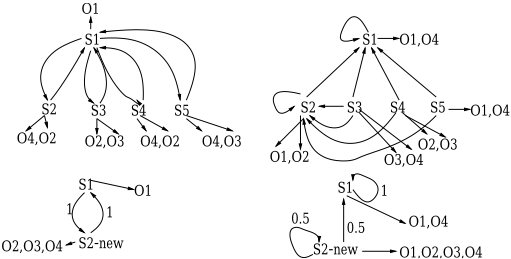
An example of a system with 5 states, 4 observations and two actions, in which a simple linear dependence can be seen, is provided in Figure 1. The model corresponding to action a is in the upper left while the model for action b is in the upper right. The solid lines represent state transitions and the dashed lines represent emission probabilities. For action a, from state S1 the system transitions to one of the other states with equal probability. These states return deterministically to S1. Under action b, from all the bottom states the system transitions with probability 0.5 to state S1. The observations can be assumed to have all the same probability, although this does not really matter for the example. In this case, states S3, S4 and S5 are all linearly dependent on S2 (they have the same transition probabilities). However, note that they do not have the same observation models. The bottom row presents a simplified system, which has been reduced to two states by eliminating the linearly dependent states. The models for action a and b are in the left and right column. The emission probabilities are all equal when more than one observation is emitted from a state. In general, these probabilities would be computed by averaging the emission probabilities for the states in the original model.

Note that this theorem relates only linearly dependent state transitions to PSR compression without considering the observations. In fact, more compression can be obtained if the observations are taken into account. A good example of this sort is the POMDP coffee domain used in [Poupart and Boutilier, 2003]. This problem has 32 states, 2 actions and 3 observations. Four of these states are linearly dependent on the other ones, which means that the dimensionality can be reduced to 28. However, by running the linear PSR construction algorithm, a more significant reduction is possible: the problem can be represented with just two tests. The value-directed compression method of [Poupart and Boutilier, 2003] takes advantage of the same regularities as linear PSRs, but also of regularities in the reward function.