
A Simple-Transition Model for Relational Sequences
Proceedings of the Nineteenth International Joint Conference on Artificial Intelligence. Pages 696-700.
© 2005 International Joint Conferences on Artificial Intelligence
Abstract
We use “nearly sound” logical constraints to infer hidden states of relational processes. We introduce a simple-transition cost model, which is parameterized by weighted constraints and a statetransition cost. Inference for this model, i.e. finding a minimum-cost state sequence, reduces to a single-state minimization (SSM) problem. For relational Horn constraints, we give a practical approach to SSM based on logical reasoning and bounded search. We present a learning method that discovers relational constraints using CLAUDIEN [De Raedt and Dehaspe, 1997] and then tunes their weights using perceptron updates. Experiments in relational video interpretation show that our learned models improve on a variety of competitors.
- [Amit et al., 1989] D. Amit, K. Wong, and C. Campbell. Percep- tron learning with sign-constrained weights. Journal of Physics A: Mathematical and General, 22:2039-2045, 1989.
- [Collins, 2002] M. Collins. Discriminative training methods for hidden Markov models: Theory and experiments with the per- ceptron algorithm. In Conf. on Empirical Methods in NLP, 2002.
- [De Raedt and Dehaspe, 1997] L. De Raedt and L. Dehaspe. Clausal discovery. Machine Learning, 26:99-146, 1997.
- [De Raedt and Kersting, 2004] L. De Raedt and K. Kersting. Prob- abilistic logic learning. ACM-SIGKDD Explor., 5, 2004.
- [Dechter, 1999] R. Dechter. Bucket elimination: A unifying frame- work for reasoning. AIJ, 113(1-2), 1999.
- [Fern and Givan, 2004] A. Fern and R. Givan. Relational sequential inference with reliable observations. In ICML, 2004.
- [Fern, 2004] Alan Fern. Learning Models and Formulas of a Tem- poral Event Logic. PhD thesis, Purdue University, August 2004.
- [Forney, 1973] G. Forney. The Viterbi algorithm. Proceedings of the IEEE, 61(3):268-278, 1973.
- [Jaumard and Simeone, 1987] B. Jaumard and B. Simeone. On the complexity of the maximum satisfiability problem for Horn for- mulas. Information Processing Letters, 26:1-4, 1987.
- [Jiang et al., 1995] Y. Jiang, H. Kautz, and B. Selman. Solving problems with hard and soft constraints using a stochastic algo- rithm for MAX-SAT. In Joint Workshop on AI and OR, 1995.
- [Lafferty et al., 2001] J. Lafferty, A. McCallum, and F. Pereira. Conditional random fields: Probabilistic models for segmenting and labeling sequence data. In ICML, pages 282-289, 2001.
- [Murphy, 2002] Kevin Murphy. Dynamic Bayesian Networks: Rep- resentation, Inference and Learning. PhD thesis, UC Berkeley, Computer Science, July 2002.
- [Ostendorf et al., 1996] M. Ostendorf, V. Digalakis, and O. Kim- ball. From HMMs to segment models: a unified view of stochas- tic modeling for speech recognition. IEEE Trans. on Speech and Audio Proc., 1996.
- [Papadimitriou, 1995] Christos H. Papadimitriou. Computational Complexity. Addison-Wesley Publishing, 1995.
- [Rosenblatt, 1958] F. Rosenblatt. The Perceptron: A probabilistic model for information storage and organization in the brain. Psy- chological Review, 65:386-408, 1958.
- [Sanghai et al., 2003] S. Sanghai, P. Domingos, and D. Weld. Dy- namic probabilistic relational models. In IJCAI, 2003. IJCAI
- [Siskind, 2001] J. Siskind. Grounding lexical semantics of verbs in visual perception using force dynamics and event logic. JAIR, 15:31-90, 2001.
- [Siskind, 2003] J. Siskind. Reconstructing force-dynamic models from video sequences. AIJ, 151(1-2):91-154, 2003.
- [Taskar et al., 2002] B. Taskar, P. Abbeel, and D. Koller. Discrimi- native probabilistic models for relational data. In UAI, 2002.
- [Veksler, 1999] O. Veksler. Efficient Graph-based Energy Mini- mization Methods in Computer Vision. PhD thesis, Cornell Uni- versity, Computer Science, July 1999.
- [Wellman et al., 1992] M. Wellman, J. Breese, and R. Goldman. From knowledge bases to decision models. Knowledge Engi- neering Review, 5, 1992.
References were extracted automatically from the PDF and may contain errors.
Full text extracted automatically from the PDF; figures, tables and equations may differ. The PDF is the version of record.
1 Introduction
We consider hidden-state inference from the observations of relational processes, i.e. processes where states and observations are described by properties of and relations among objects (e.g. people and blocks). To deal with the enormous state and observation spaces, we utilize "nearly-sound" (i.e. rarely violated) logical constraints on the states and observations. Such constraints can often be acquired via machine learning and/or a human expert, and we give a framework for combining them for relational sequential inference.
We introduce the simple-transition cost model (in Section 3), which is parameterized by a set of weighted logical constraints and a state-transition cost. The cost of a state sequence given an observation sequence is the weight of unsatisfied constraints plus a transition cost for each state change. Sequential inference corresponds to computing the minimum-cost state sequence. Here we study both learning and inference for this model.
First, in Section 4, we (efficiently) reduce sequential inference to a single-state minimization (SSM) problem. We then show, in Sections 5 and 6, how to leverage nearly-sound relational Horn constraints in order to compute SSM with practical efficiency. We also study the possibility of exploiting efficient SSM in richer models. We show that for a simple enrichment to our model, there is no efficient reduction unless P=NP. In Section 7, we discuss learning a relational simpletransition model using the logical discovery engine CLAUDIEN [De Raedt and Dehaspe, 1997] and a variant of Collins'
generalized perceptron algorithm [Collins, 2002]. Finally, in Section 8, we evaluate our approach in a relational videointerpretation domain. Our learned models improve on the accuracy of an existing trainable system and an approach based on more mainstream approximate inference.
2 Problem Setup
For simplicity, we describe our problem setup and approach for propositional (rather than relational) processes, where in the spirit of dynamic Bayesian networks (DBNs) [Murphy, 2002], states are described by a fixed set of variables. In Section 6, we extend to the relational setting.
A sequential process is a triple (X, Y,P), where the observation space X and state space Y are sets that contain all possible observations and states. P is a probability distribution over the space of finite sequences constructed from members of X × Y. Each such sequence contains a pair of an observation sequence (o-sequence) and a state sequence (s-sequence). For a sequence Q = (q1, . . . , qT ), we let Qi:j = (qi, . . . , qj) for i ≤ j. We will use uppercase for sequences and lowercase for single states and observations. A process is propositional when its states are represented using a set of n state variables over the finite domain Ds, yielding Y = (Ds)n . The value of the i'th variable in state s is denoted by s(i) . We will not need to assume a representation for observations until Section 6
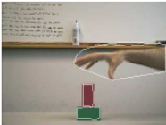
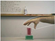
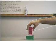
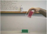
We assume that the utility of an inferred s-sequence S primarily derives from the sequence of distinct states, rather than identifying the exact state transition points. Let COMPRESS(S) denote the sequence obtained by removing consecutive repetitions in S. For example, COMPRESS(a, a, a, b, b, a, c, c) = a, b, a, c. Our empirical goal is to map an o-sequences O to an s-sequence S such that COMPRESS(S) is the distinct sequence of states that generated O. Indeed, in our video domain, the exact locations of state transitions are often ambiguous (as judged by a human) and unimportant for recognizing activity-e.g. in Figure 1 it is unimportant to know exactly where the transition occurs.
Example 1. The process in our video-interpretation domain corresponds to a hand playing with blocks. Figure 1 shows key frames where a hand picks up a red block from a green block. The goal is to observe the video and then infer the underlying force-dynamic states, describing the support relations among objects. States are represented as sets of forcedynamic facts, such as ATTACHED(HAND, RED). Observations are represented as sets of low-level numeric facts, such as DISTANCE(GREEN, RED) = 3, that are derived from an object tracker's noisy output. For a fixed set of objects, the process can be represented propositionally with a variable for each possible fact. However, our system must handle any number of objects, requiring a relational process representation described in Section 6.
Frame 21
Figure 1: Key frames in a video segment showing a hand picking up a red block from a green block. The object tracker's output is shown by the polygons. The video segment has two distinct force-dynamic states given by: {GROUNDED(HAND), GROUNDED(GREEN), CONTACTS(GREEN, RED)} (frames 1 and 3) and {GROUNDED(HAND), GROUNDED(GREEN), ATTACHED(HAND, RED)} (frames 14 and 20). The transition occurs between frames 3 and 14. See Example 2 regarding the predicates GROUNDED, CONTACTS, and ATTACHED.
3 The Simple-Transition Cost Model
Our framework utilizes an additive conditional cost model C(S|O) to represent the cost of labeling o-sequence O1:T by s-sequence S1:T
with real-valued atemporal-cost and transition-cost functions Ca and Ct. This is the cost cost model implicit in (conditional) hidden Markov models (HMMs). Ca(si|oi) is the cost of labeling oi by state si, and Ct(si, si-1) is the cost of transitioning from state si-1 to si. As in [Lafferty et al., 2001], our work extends to Ca's with "non-local" observation dependencies. Sequential inference involves computing arg minS1:T C(S1:T |O1:T ) for a given O1:T .
C(S1:T |O1:T ) is a simple-transition model (STM) with parameters 〈Ca,K〉 if the atemporal-cost function is Ca and Ct(si, si-1)=K·δ(si ̸= si-1), where K is a real, and δ(p) = 1 if p is true else 0. This model charges an equal cost for all state transitions, even though generally some transitions types are more likely than others. If this likelihood information is critical for inference, then an STM alone will not suffice. However, we believe that there are interesting processes where accurate inference does not require exploiting non-simple transition structure. For example, in our video domain, states persist for many observations and can be reliably inferred by integrating just those observations, without considering transition type. For such processes, it is important to study simple but sufficient models, as there can be considerable computational advantages.
4 Inference for Simple-TransitionModels
Viewing an STM as an HMM we can apply the Viterbi algorithm [Forney, 1973] to compute a minimum-cost s-sequence S1:T in O(T · |Y|2 ) time. In fact, by leveraging the simpletransition structure, Viterbi can be improved to O(T · 2 · |Y|) time. However, these algorithms are impractical for us since they are exponential in the number of state variables n (i.e. |Y| = |Ds|n ), which will typically be large for our relational processes. Likewise, for STMs, general-purpose graphical-modeling techniques such as variable elimination and junction-tree algorithms are exponential in n (i.e. the induced tree width [Dechter, 1999] is linear in n).
Reduction to SSM. Sequential inference for an STM 〈K, Ca〉 reduces to the single-state minimization (SSM) problem, which is defined as computing the SSM function σ(O1:j) = mins ∑1≤i≤j Ca(s|oi). The SSM function gives the minimum cost of labeling O1:j by a single state (i.e. no state transitions). For an o-sequence O1:T we denote the minimum cost over all s-sequences as C ∗ (O1:T ) = minS1:T C(S1:T |O1:T ). For STMs, C ∗ (O1:T ) can be expressed in terms of σ as follows (for proof see Fern [2004]).
Equation 2 minimizes over j, where j + 1 is viewed as the final state-transition point. The minimum cost over ssequences with final transition j + 1 equals the minimumcost sequence up to j, plus a transition cost K (unless j=0), plus the SSM cost for the remaining suffix (no transitions occur after j). This decomposition is possible because STMs weigh all transition types equally, decoupling the minimization problems before and after j.
Equation 2 yields an efficient reduction to SSM based on dynamic programming, which we call the SSM-DP algorithm. Simply compute C ∗ (O1:j) in the order j = 1, 2, . . . , T for a total of T 2 SSM computations. It is straightforward to store information for extracting the minimum-cost ssequence, which we denote by SSM-DP(O1:T , σ,K). Thus, efficient SSM computation implies efficient sequential inference for STMs. The complexity of SSM depends on the particular representation used for Ca. In Section 5, we leverage nearly-sound logical constraints to provide practically efficient SSM.
Though SSM-DP provides the potential for handling large state spaces, a naive implementation requires T 2 SSM computations, which is often unacceptable. However, significant and sound pruning of the computation is possiblee.g. in Equation 2, ignore any j when a k exists such that C(S1:k|O1:k) ≤ C(S1:j|Oi:j) + σ(Oj+1:k). In our application, pruning reduces the empirical number of SSM computations to O(T). See Fern [2004] for details.
Sufficient SSMComputation. In practice we do not need exact SSM for all o-sequences. Rather we need only to compute a sufficient SSM approximation defined below. O1:j is a critical o-sequence of process P if for some o-sequence drawn from P, O1:j is a maximal subsequence generated by a single state. Let σ be the SSM function for an STM
that accurately predicts s-sequences of P. We say σ′ is a sufficient SSM approximation to σ for P if both 1) for all o-sequences O1:T , σ(O1:T ) ≤ σ′ (O1:T ), and 2) σ′ (O′ ) = σ(O′ ) for any critical o-sequence O′ of P. It can be shown that for o-sequences drawn from P, SSM-DP(O1:T , σ, K) = SSM-DP(O1:T , σ′ ,K). Thus we can achieve accurate inference using σ′ . In Section 5 we show how to efficiently compute such an approximation.
Non-Simple Models. Given our focus on SSM it is natural to consider efficient SSM reductions for non-simple models. Intuitively, if a model distinguishes between different transition types, we may need to consider states other than just SSM solutions (like Viterbi but unlike SSM-DP), possibly resulting in exponential behavior in n even given efficient SSM. Below we show that an efficient reduction is unlikely for a modest extension to STMs, giving a boundary between efficient and inefficient models under efficient SSM.
We extend STMs by allowing the model to assign higher costs to transitions where more state variables change, unlike STMs which can only detect whether a change occurred. A cost model C, with atemporal component Ca, is a countingtransition model if Ct(si, si-1) = K · ∑1≤j≤n δ(s(j) i ̸= s(j) i-1 ), i.e. transition cost is linear in the count of propositions that change. We say C allows efficient SSM if the SSM function for Ca is computable in time polynomial in its input osequence size and number of state variables.
Theorem 1. Given as input a counting-transition model C, an observation sequence O, and a cost bound τ, the problem of deciding whether C ∗ (O1:T ) < τ is NP-complete, even under the assumption that C allows efficient SSM.
Proof: (sketch) See Fern [2004] for full proof. Inference in 2-d grid Potts models, a class of Markov random fields, is NPhard [Veksler, 1999]. We first give a non-trivial extension of this result to the smaller class of 2-d grid Potts models with equally weighted "horizontal edges". Next, we reduce this problem to counting-transition model inference. Intuitively, the state variables at time i represent the Potts model nodes in column i. Finally, we show that the constructed model allows efficient SSM via variable elimination. ✷
5 Constraint-Based SSM
We now give a constraint-based representation for atemporalcost functions and study the corresponding SSM problem. For simplicity, we assume that states have n binary state variables, i.e. Ds = {true, false}. We also assume a set of m binary observation tests, each one mapping observations to {true, false}. Non-binary extensions are straightforward.
Propositional Horn Constraints. A propositional Horn constraint φ is a logical implication (body → head), where body is a conjunction of state variables and observation tests, and head is a state variable or false. Given an observation o and state s, we let φ[o] (φ[s]) denote the result of substituting observation tests (state variables) in φ with the truth values under o (under s). If a constraint has no variables, then it is interpreted as the truth value of the variable-free expression. Thus, φ[o][s] is the truth value of φ under o and s, and we say that o and s satisfy φ iff φ[o][s] is true. A set of Horn constraints is satisfiable iff there exists a state and observation that jointly satisfy each constraint. For horn constraints, testing satisfiability and finding satisfying assignments are polynomial-time computable [Papadimitriou, 1995].
Constraint-Based Cost Functions. We parameterize an atemporal-cost function using a set of weighted Horn constraints Φ = {〈φ1, c1〉, . . . , 〈φv, cv〉}, with Horn constraints φi and non-negative weights ci representing the cost of violating φi. The non-negativity requirement will be important for inference. The sum of costs in Φ is denoted by COST(Φ) and we say Φ is satisfiable if its set of constraints is satisfiable. Atemporal cost is defined as Ca(s|o,Φ) = ∑〈φ,c〉∈Φ c · δ(¬φ[o][s]), i.e. the total cost of unsatisfied constraints. In this work, we will assume that Φ contains "nearly sound" constraints, meaning that each constraint is usually satisfied by the state/observation pairs generated by our process. Our primarily non-theoretical goals do not require a formal notion of nearly sound (e.g. PAC).
Given Φ and an o-sequence O1:j , we define the combined constraint set as Γ(O1:j,Φ) = ⋃1≤i≤j ⋃〈φ,c〉∈Φ 〈φ[oi], c〉, which involves only state variables and captures all of the state constraints "implied" by Φ and O1:j. The SSM function for Ca is now given by
which is equivalent to solving maximum satisfiability (MAX-SAT) [Jiang et al., 1995] for Γ(O1:j , Φ), where MAXSAT asks for an s such that the weight of satisfied constraints is maximum. While the number of SSM variables is fixed, the constraint set grows with sequence length. Fortunately, in practice we can significantly reduce this set by pruning and merging. PRUNE(Φ) contains members of Φ that do not have false in the constraint's body. MERGE(Φ) combines logically equivalent members of Φ into one constraint by summing weights. MAX-SAT solutions are invariant under both operators. Thus, we solve SSM via MAX-SAT for the smaller constraint Γ∗ (O1:j , Φ) = MERGE(PRUNE(Γ(O1:j , Φ))).
A Dual MAX-SAT Approach. MAX-SAT is NP-hard even for Horn constraints [Jaumard and Simeone, 1987]. Rather than use general-purpose approximate techniques, we give a MAX-SAT approach that leverages our setting of nearly-sound Horn constraints. Let π = Γ∗ (O1:j,Φ) and Π be the set containing all satisfiable subsets of π. An equivalent dual form of Equation 4 is σ(O1:j|Φ) = COST(π) - maxπ′∈Π COST(π′ ), which asks for a maximum-cost member of Π. This motivates the following MAX-SAT approach that searches through constraint subsets rather than than variable assignments. Conduct a cost-sensitive breadthfirst search through subsets of π for a satisfiable subset-i.e. starting at π consider π subsets in order of non-increasing cost until finding a satisfiable one. Any satisfying assignment for this set is a MAX-SAT solution provided all weights are non-negative. For negative weights a satisfying assignment for a consistent constraint set may not be a MAX-SAT solution. Although we can always replace a negatively weighted constraint 〈φ, c〉 by 〈¬φ,-c〉, ¬φ may not be horn, possibly making SAT hard. Hence we require non-negative weights.
Since testing satisfiability is efficient for Horn constraints, the time required by the dual approach primarily depends on the number of search nodes we consider. This number is bounded by the number of subsets of π that have a cost greater than σ(O1:j|Φ), which can be exponentially large. Thus, we compute an approximation στ to σ by first searching through subsets of π for a maximum of τ steps. We return a solution if one is found and otherwise return an upper-bound to σ(O1:j |Φ) resulting from a greedy hill-climbing search.
| ATTACHED(x, y) GROUNDED(x) CONTACTS(x, y) | x supports y by attachment support of x is unknown x supports y by contact |
| DIRECTION(x,d) SPEED(x,s) ELEVATION(x,e) MORPH(x,c) DISTANCE(x,y,d) ∆DIST(x,y,dd) COMPASS(x,y,c) ANGLE(x,y,a) | x is moving in direction d x's speed is s x's elevation is e x's shape-change factor is c distance between x and y is d change in distance is dd compass direction of y to x is c angle between x and y is a |
Though στ will not be correct for all inputs, we know from Section 4, that it need only be a sufficient approximation to guarantee correct sequential inference. When our constraints are nearly sound, στ will tend to be sufficient even for small τ. That is, στ will equal σ for critical o-sequences. Recall that when O1:j is a critical o-sequence it must be generated by a single state s. Thus, s will satisfy most constraints in Γ∗ (O1:j , Φ) and our search need only remove a small number of constraints (the unsatisfied ones) to find a satisfiable subset. In addition, as described in the full paper, the MERGE operation tends to place high weight on the satisfied constraints, which often leads in removing unsatisfied constraints first.
6 Extending to Relational Processes
In the spirit of knowledge-base model construction [Wellman et al., 1992], we extend to relational processes by compiling "relational schemas" to propositional models and use the ideas from previous sections.
Relational Processes. A process (X, Y,P) is relational when the observation and state spaces X and Y are given by specifying a domain set of objects D, a state-predicate set Rs, and an observation-feature set Fo, each having a specified number of arguments. An observation fact has the form "f = v", where f is an observation feature applied to objects and v is a number. A state fact is a predicate fromRs applied to objects. See Example 1 for example facts from our video domain. Observations (states) are finite sets of observation (state) facts, representing all the facts that are true, and X (Y) contains all such sets. States are restricted to only involve objects that appear in the corresponding observation. We often view relational states as propositional. Given a finite D′ ⊆ D, denote by Y[D′ ] the propositional state space over n binary variables, one variable for each of the n = O(|D′ |q ) state facts involving only objects in D′ , where q is the maximum state-predicate arity.
Example 2. In our video domain we infer force-dynamic state sequences from videos of a hand playing with blocks. D contains all hands and blocks we might encounter. There are three force-dynamic state predicates and eight observation features, shown in Table 1. Figure 1 depicts two distinct force-dynamic states. Observations are sets of observation facts calculated for the objects and object pairs based on the PERCEPTRON(TRN, {φ1, . . . , φv}, τ,M) K ← 0; ⃗C =⃗0; repeat M times, for-each 〈O, S〉 ∈ TRN Φ ← {〈φ1, c1〉, . . . , 〈φv, cv〉} ˆ S ← SSM-DP(O, στ r (·|Φ), K) if ˆ S ̸= S, ⃗C ← [ ⃗C + ⃗V ( ˆ S, O) - ⃗V (S, O)]+ K ← [K + TRANS( ˆ S) - TRANS(S)]+
return 〈 ⃗C, K〉
Figure 2: Generalized Perceptron Pseudocode. [ ⃗C]+ = ⃗C ′ s.t. c′i =max(0, ci).
object tracker output.
Relational Horn Constraints. A state atom is a state predicate or the relation "̸=" applied to variables. An observation atom has the form "(f1 r f2)", where r ∈ {=,≤}, and fi is a number or an observation feature applied variables. A relational Horn constraint has the form (body → head), where body is a conjunction of state and/or observation atoms, and head is a state atom or false and may only contain variables that appear in body. For example, (DISTANCE(x, y) ≤ 5) ∧ (6 ≤ Speed(y)) → ATTACHED(x, y) is a relational Horn constraint for predicting object attachment based on an observation. A relational Horn constraint φ is a schema for propositional constraints. Any way of (consistently) replacing variables in φ with objects gives a (propositional) ground instance of φ. Given a set of objects D′ , GROUND(φ,D′ ) contains all ground instances with only objects in D′ .
Relational Cost Models. A relational simple-transition model is a pair 〈Φ,K〉, with transition-cost K and nonnegatively weighted relational Horn constraints Φ = {〈φ1, c1〉, . . . , 〈φv, cv〉}. Given a relational o-sequence O1:T with objects D′ , we know that states may only involve facts constructed from D′ , and thus we need only consider the propositional state space Y[D′ ]. To infer an s-sequence over Y[D′ ] we use the set of propositional constraints Φp = ⋃〈φ,c〉∈Φ ⋃φ′∈GROUND(φ,D′) 〈φ′ , c〉 to define an atemporal cost function Ca(s|o,Φp) as in Section 5. We then return the lowest-cost S1:T given by SSM-DP(O1:T , στ r (·|Φ), K), where στ r (O1:j |Φ) = στ (O1:j |Φp) is a relational SSM function with search bound τ. That is στ r is computed by compilation to a propositional SSM function στ and then using our bounded-search dual MAX-SAT approach.
A naive implementation of this approach can be expensive since Φp can be large. Fortunately, in practice, our relational representation allows us to avoid constructing most of the set. We use efficient forward-chaining logical inference to construct Γ∗ (O1:T ,Φp), the input to MAX-SAT, without explicitly constructing Φp. Space constraints preclude details.
7 Learning a Relational STM
We learn relational STMs by first running the relational learner CLAUDIEN [De Raedt and Dehaspe, 1997] on a training set of labeled o-sequences, acquiring "nearly sound" relational Horn constraints that are satisfied by the training data (producing 300-400 constraints for our domain). Next, using a new training set we jointly tune the constraint weights and transition-cost K using a variant of Collins' voted perceptron algorithm [Collins, 2002]. The algorithm extends Rosenblatt's perceptron for binary labels [Rosenblatt, 1958] to handle structured labels such as sequences, and has convergence and generalization properties similar to Rosenblatt's.
The algorithm requires representing cost using a linear combination of n features, which we do as follows. Given O1:T and S1:T involving just objects in the finite D′ , and a relational STM 〈{〈φ1, c1〉, . . . , 〈φv, cv〉},K〉, the violation-count feature of φi is Vi(O1:T , S1:T ) = ∑1≤i≤T ∑φ′∈GROUND(φi,D′) δ(¬φ′ [oi][si]), i.e. the number of unsatisfied instances of φi. We let ⃗V (O1:T , S1:T ) be the v-dimensional vector of violation-count features and ⃗C = [c1, . . . , cv] is the weight vector. The transition count feature TRANS(S1:T ) is equal to the number of state transitions in S1:T . These v + 1 features represent the STM cost as C(S1:T |O1:T ) = ⃗V (O1:T , S1:T ) · ⃗C + TRANS(S1:T ) · K.
The algorithm (see Figure 2) cycles through the training data and when an incorrect s-sequence ˆ S is inferred in place of S, the weights are adjusted to increase cost for ˆ S and decrease cost for S. The input is a training set TRN, relational Horn constraints {φ1, . . . , φv}, an SSM search bound τ , and the number M of iterations. The output is the learned weights ⃗C and transition cost K. Ideally we want this STM to allow for accurate sequential inference when using the searchbounded relational SSM function στ r . Unlike Collins we require non-negative weights for inference. Thus, we set a weight to zero if a normal perceptron update would result in a negative value. This variant has not yet been shown to possess the convergence and generalization properties of the unconstrained version. However, this variant of Rosenblatt's perceptron has been shown to converge [Amit et al., 1989].
8 Experimental Results
We apply our technique to force-dynamic state inference from real video. The LEONARD system [Siskind, 2001] uses these states to recognize events, such as "a hand picked up a block" (see Figure 1). Recently [Fern and Givan, 2004] developed a trainable system for this problem using the forward greedy merge (FGM) algorithm, which outperformed prior techniques. FGM also utilizes Horn constraints, but assumes that they are sound, rather than nearly sound. Since this is not true for CLAUDIEN-learned constraints, which were also used by FGM, that work utilized two steps to improve performance: 1) Constraint pruning yields a much smaller but (hopefully) "sufficient" constraint set, reducing the chance of constraint violations. 2) Sequence-cleaning preprocessing is an ad-hoc step that removes observations where constraint violations are "detected". See [Fern and Givan, 2004] for details. While these steps allowed for good performance, the soundness assumption limits the approach's applicability, as such preprocessing will not always be effective. The motivation for the work in this paper was to develop a "softened" more robust framework for utilizing nearly-sound constraints.
Procedure. Our corpus of 210 videos from [Siskind, 2003] contains 7 event types (30 movies each) involving a hand playing with up to three blocks (e.g. assembling a tower). We use the hand-labeled training sets of size 14 (TRN-14) and 21 (TRN-21) from [Fern and Givan, 2004]. The remaining videos are labeled with their compressed s-sequences (the output of COMPRESS), which is the label we wish to predict.
For each training set, we learn relational STMs for three SSM search bounds τ = 0, 100, 1000. Seven training instances are used by CLAUDIEN to acquire constraints and the perceptron algorithm is run for 100 iterations on the remaining instances. We evaluate each iteration's model according to the % of test videos for which SSM-DP's compressed inferred s-sequence is correct (using the same τ as for learning).
We compare against FGM used with an without sequence cleaning and always with pruning. We also compare against a system that is closer to mainstream graphical modeling techniques, which uses the counting-transition model of Section 4, and WALKMAXSAT [Jiang et al., 1995] for approximate inference. The model is identical to our relational STMs, using the same CLAUDIEN-learned constraints, except that it has a non-simple transition structure. For sequential inference we construct a single large MAX-SAT problem corresponding to the transition-counting model and use WALKMAXSAT to find an approximate solution. We tune the model's weights using the perceptron algorithm with WALKMAXSAT (rather than SSM-DP) for inference.
Performance Across Iterations. Table 2 shows, for each training set, the testing error of our learned STMs for τ = 0, 100, 1000 (shown as SSM-DP(τ)), over the first eight perceptron iterations. There is always a rapid improvement after iteration one, followed by a period of fluctuating or constant performance. The fluctuation continues out to iteration 100 (not shown), but never improves over the best performance shown. In practice, one could use cross-validation to select a good model, or consider "weight averaging" [Collins, 2002]. Note that the best performance on the smaller training set TRN-14 is superior to TRN-21. Our explanation for this is that by using relatively small training sets, the results can be significantly affected by a small number of particularly noisy movies (presumably in TRN-21). Experiments not shown, provide evidence for this by training on subsets of TRN-21. 1
Bounding Search. The search bound τ = 0 means that SSM is (approximately) solved via hill-climbing. Surprisingly we can learn weights for which hill-climbing performs well. Increasing the search bound improves performance with respect to the best model across iterations, particularly for TRN-14. The last column shows the frames processed per second when inferring states for our corpus. Inference time apparently does not increase linearly with τ, indicating that the SSM search typically end much before reaching the bound. Increasing τ to 10,000, doubles inference time, but neither improves nor hurts results.
Other Techniques. We significantly outperform WALKMAXSAT (further iterations did not help), which we allowed a generous search time, using search cutoff 106 with 103 random restarts (other settings did not improve). Further experiments suggest that WALKMAXSAT does not scale well for our problems. Using learned STM weights for the countingtransition model, WALKMAXSAT reliably infers correct ssequences for short videos, but is very poor for long videos. WALKMAXSAT gave equally poor results when used to learn STMs rather than counting-transition models. This suggests the poor performance is primarily due to the ineffectiveness of this general-purpose inference technique for our models. We conjecture that other approximate techniques such as (loopy) belief propagation and Gibbs sampling will also yield inferior performance. Indeed, Gibbs sampling is very similar to WALKMAXSAT. Evaluating this conjecture is future work.
1 Runtime of CLAUDIEN (interpreted Prolog) on TRN-21 was about six days. Thus, it was not feasible to average results across many training sets. In another full experiment (21 movies), we observed similar (slightly better) performance for SSM-DP, and similar relative performance to the other systems.
| TRN-14 (Iteration) | TRN-21 (Iteration) | FPS | |||||||||||||||
|---|---|---|---|---|---|---|---|---|---|---|---|---|---|---|---|---|---|
| 1 | 2 | 3 | 4 | 5 | 6 | 7 | 8 | 1 | 2 | 3 | 4 | 5 | 6 | 7 | 8 | ||
| SSM-DP(0) | 94 | 24 | 3.2 | 2.1 | 2.1 | 2.6 | 2.1 | 2.6 | 94 | 6.3 | 6.9 | 5.8 | 4.8 | 12 | 17 | 3.7 | 15 |
| SSM-DP(100) | 93 | 32 | 2.6 | 2.6 | 2.1 | 2.1 | 2.1 | 2.1 | 93 | 3.2 | 3.7 | 3.7 | 3.2 | 10 | 21 | 8.5 | 14 |
| SSM-DP(1000) | 93 | 31 | 4.2 | 1.6 | 1.1 | 1.1 | 1.1 | 1.1 | 93 | 3.2 | 3.7 | 3.7 | 3.2 | 10 | 21 | 8.5 | 8 |
| WALKMAXSAT | 96 | 46 | 51 | 54 | 50 | 43 | 50 | 58 | 95 | 47 | 50 | 60 | 49 | 50 | 45 | 52 | 1.4 |
| FGM / FGM+SC | 17 / 6.3 | 3.2 | 29 | ||||||||||||||
FGM without sequence cleaning (shown as FGM) is an order of magnitude worse than STMs (which never use cleaning). We significantly improve on FGM with sequence cleaning (FGM+SC) on TRN-14 and yield equal performance on TRN-21. FGM is faster, close to frame rate. A reimplementation of our LISP prototype will likely achieve frame rate.
9 RelatedWork
Segment models [Ostendorf et al., 1996] subsume our STM formulation. We are not aware of prior work that has leveraged or noted the SSM reduction for large state spaces. Perhaps this is because prior segment modeling work typically utilizes non-simple transition structure (perhaps sometimes unnecessarily) and to our knowledge has not been applied to large state spaces.
Our "model schema" approach for handling relational data is now standard in probabilistic modeling [De Raedt and Kersting, 2004]. Most closely related are relational Markov networks (RMNs) [Taskar et al., 2002]. A relational STM can be viewed as defining a log-linear conditional RMN, where the RMN "clique feature templates" correspond to relational Horn constraints and a transition template. RMNs are very general and thus the existing techniques do not fully exploit the structure of relational STMs. Instead RMN-like proposals rely on general-purpose approximate inference (e.g. belief propagation), with unclear practical implications. Likewise dynamic probabilistic relational models [Sanghai et al., 2003] provide a generic schema-based approach specialized to relational sequence data. Again the generality precludes leveraging the STM structure.
Acknowledgments
This work was supported in part by NSF grants 9977981-IIS and 0093100-IIS.
@inproceedings{ijcai2005p31,
  title     = {A Simple-Transition Model for Relational Sequences},
  author    = {Fern, Alan},
  booktitle = {Proceedings of the Nineteenth International Joint Conference on
               Artificial Intelligence, {IJCAI-05}},
  publisher = {International Joint Conferences on Artificial Intelligence},
  editor    = {Leslie Pack Kaelbling and Alessandro Saffiotti},
  pages     = {696--700},
  year      = {2005},
  url       = {https://ijcai.org/proceedings/2005/31},
}
TY - CPAPER TI - A Simple-Transition Model for Relational Sequences AU - Fern, Alan T2 - Proceedings of the Nineteenth International Joint Conference on Artificial Intelligence, IJCAI-05 PB - International Joint Conferences on Artificial Intelligence PY - 2005 SP - 696 EP - 700 UR - https://ijcai.org/proceedings/2005/31 ER -Copied
Machine-readable versions of this paper, for tools and AI agents:





