
Word Sense Disambiguation with Distribution Estimation
Proceedings of the Nineteenth International Joint Conference on Artificial Intelligence. Pages 1010-1014.
© 2005 International Joint Conferences on Artificial Intelligence
Abstract
A word sense disambiguation (WSD) system trained on one domain and applied to a different domain will show a decrease in performance. One major reason is the different sense distributions between different domains. This paper presents novel application of two distribution estimation algorithms to provide estimates of the sense distribution of the new domain data set. Even though our training examples are automatically gathered from parallel corpora, the sense distributions estimated are good enough to achieve a relative improvement of 56% when incorporated into our WSD system.
- [Agirre and Martinez, 2004] E. Agirre and D. Martinez. Un- supervised WSD based on automatically retrieved ex- amples: The importance of bias. In Proceedings of EMNLP04, pages 25-32, Barcelona, Spain, July 2004.
- [Efron and Tibshirani, 1993] B. Efron and R. J. Tibshirani. An Introduction to the Bootstrap. Chapman & Hall, New York, 1993.
- [Escudero et al., 2000] G. Escudero, L. Marquez, and G. Rigau. An empirical study of the domain dependence of supervised word sense disambiguation systems. In Pro- ceedings of EMNLP/VLC'00, Hong Kong, October 2000.
- [Kilgarriff, 2001] A. Kilgarriff. English lexical sample task description. In Proceedings of SENSEVAL-2, pages 17-20, Toulouse, France, July 2001.
- [Lee and Ng, 2002] Y. K. Lee and H. T. Ng. An empiri- cal evaluation of knowledge sources and learning algo- rithms for word sense disambiguation. In Proceedings of EMNLP02, pages 41-48, Philadelphia, Pennsylvania, USA, July 2002.
- [McCarthy et al., 2004a] D. McCarthy, R. Koeling, J. Weeds, and J. Carroll. Automatic identification of infrequent word senses. In Proceedings of COLING04, pages 1220-1226, Geneva, Switzerland, August 2004.
- [McCarthy et al., 2004b] D. McCarthy, R. Koeling, J. Weeds, and J. Carroll. Finding predominant word senses in untagged text. In Proceedings of ACL04, pages 280-287, Barcelona, Spain, July 2004.
- [Miller, 1990] G. A. Miller. Wordnet: An on-line lex- ical database. International Journal of Lexicography, 3(4):235-312, 1990.
- [Ng et al., 2003] H. T. Ng, B. Wang, and Y. S. Chan. Ex- ploiting parallel texts for word sense disambiguation: An empirical study. In Proceedings of ACL03, pages 455-462, Sapporo, Japan, July 2003.
- [Och and Ney, 2000] F. J. Och and H. Ney. Improved statis- tical alignment models. In Proceeedings of ACL00, pages 440-447, Hong Kong, October 2000.
- [Palmer et al., 2001] M. Palmer, C. Fellbaum, and S. Cotton. English tasks: All-words and verb lexical sample. In Pro- ceedings of SENSEVAL-2, pages 21-24, Toulouse, France, July 2001.
- [Pedersen et al., 2004] T. Pedersen, S. Patwardhan, and J. Michelizzi. Wordnet::similarity -measuring the relat- edness of concepts. In Proceedings of AAAI04, Intelligent Systems Demonstration, San Jose, CA, July 2004.
- [Saerens et al., 2002] M. Saerens, P. Latinne, and C. De- caestecker. Adjusting the outputs of a classifier to new a priori probabilities: A simple procedure. Neural Com- putation, 14(1):21-41, January 2002.
- [Vucetic and Obradovic, 2001] S. Vucetic and Z. Obradovic. Classification on data with biased class distribution. In Proceedings of ECML01, pages 527-538, Freiburg, Ger- many, September 2001.
References were extracted automatically from the PDF and may contain errors.
Full text extracted automatically from the PDF; figures, tables and equations may differ. The PDF is the version of record.
1 Introduction
Many words have multiple meanings. The process of identifying the sense of a word in a particular context is known as word sense disambiguation (WSD). WSD is an important task of natural language processing (NLP), and is important for applications such as machine translation and information retrieval. Past research has shown that a good approach to WSD is the use of supervised machine learning. With this approach, a large text corpus in which each ambiguous word has been annotated with the correct sense has to be collected to serve as training data.
The work of these researchers showed that the different sense distributions across domains have an important effect on WSD accuracy. Therefore, estimation of the target domain's sense distribution will be crucial, in order to build WSD systems that are portable across different domains. A partial solution to this would be to determine the predominant, or most frequently occurring sense of each word in a corpus. Research has shown that the baseline heuristic of selecting the most frequently occurring sense of a word gives high WSD accuracy. This is due to the often skewed distribution of word senses. McCarthy et al. [2004b] addressed this when they presented a method to automatically rank word senses in a corpus, in order to determine the predominant sense of each word. They obtained good results when the method is applied on the SENSEVAL-2 English all-words task [Palmer et al., 2001]. The same method is used in a related work [McCarthy et al., 2004a] to identify infrequently occurring word senses.
This corpus-based approach, however, raises the problem of domain dependence faced by these supervised WSD systems. A system trained on data from one domain (for example, sports), will show a decrease in performance when applied to a different domain (for example, economics). This issue of domain difference affecting WSD performance had been brought up by various researchers. Escudero et al. [2000] showed that training a WSD system in one domain and applying it to another could lead to a drop of 12% to 19% in WSD accuracy. It was shown that one of the reasons is due to different distributions of senses across domains, as a 9% improvement in accuracy was observed when they sense-balanced the instances from the different domains. Recently, Agirre and Martinez [2004] conducted experiments with training data for WSD which were automatically gathered from the Internet. They reported a potential improvement of 14% in accuracy if they have access to the sense distribution of their test data.
In the machine learning literature, algorithms to estimate class a priori probabilities have been developed. In this paper, we present novel application of two distribution estimation algorithms to provide estimates of the sense distribution, or a priori probabilities of senses, and show that they are effective in improving the WSD accuracy of systems trained and applied on different domains. Note that determining the predominant sense is a special case of trying to estimate the complete sense distribution. To the best of our knowledge, these algorithms have not been used in NLP or for WSD.
We recognize that a WSD system should be scalable. This is a problem faced by current supervised learning systems, as they usually relied on manually annotated data for training. To tackle this problem, our prior work[Ng et al., 2003] exploited parallel texts for WSD. Encouraging results were obtained in our evaluation on the nouns of SENSEVAL-2 English lexical sample task [Kilgarriff, 2001], which used the WordNet 1.7 sense inventory [Miller, 1990]. Note that the usage of parallel texts as training data represents a natural domain difference with the test data of SENSEVAL-2 English lexical sample task, of which 91% is drawn from the British National Corpus (BNC). In this paper, we chose to draw training data for our experiments from parallel texts, and similarly base our evaluation on the nouns of SENSEVAL-2 English lexical sample task.
This paper is structured as follows. In the next section, we discuss the process of gathering training data from parallel texts. In section 3, we describe the two distribution estimation algorithms used. We also give a brief description of the predominant sense method presented by [McCarthy et al., 2004b]. In section 4, we evaluate the effectiveness of the two algorithms and the predominant sense method in improving WSD accuracy. Evaluation results on the nouns in SENSEVAL-2 English lexical sample task are presented. Discussions are made in section 5, before we conclude in section 6.
| Parallel corpora | Size of English texts (in million words (MB)) | Size of Chinese texts (in million characters (MB)) |
|---|---|---|
| Hong Kong Hansards | 39.9 (223.2) | 35.4 (146.8) |
| Hong Kong News | 16.8 (96.4) | 15.3 (67.6) |
| Hong Kong Laws | 9.9 (53.7) | 9.2 (37.5) |
| Sinorama | 3.8 (20.5) | 3.3 (13.5) |
| Xinhua News | 2.1 (11.9) | 2.1 (8.9) |
| English translation of Chinese Treebank | 0.1 (0.7) | 0.1 (0.4) |
| Total | 72.6 (406.4) | 65.4 (274.7) |
2 Training Data fromParallel Texts
In this section, we briefly describe the parallel texts used in our experiments, and the process of gathering training data from them.
2.1 Parallel Text Alignment
Table 1 lists the 6 English-Chinese parallel corpora (available from Linguistic Data Consortium) used in our experiments. The sentences of the 6 corpora were already pre-aligned, either manually or automatically, when they were prepared. After ensuring the corpora were sentence aligned, we tokenized the English texts, and perform word segmentation on the Chinese texts. Next, word alignment was done on the parallel corpora using the GIZA++ software [Och and Ney, 2000].
2.2 Target Translations Selection
We took the same approach as described in our previous work [Ng et al., 2003] to select some possible Chinese translations for each sense of an English word. For instance, WordNet 1.7 lists 5 senses for the noun nature. Senses will be lumped together if they are translated in the same way in Chinese. For example, sense 2 and 3 of nature are lumped together as they are both translated as "L�l" in Chinese. Then, from the word alignment output of GIZA++, we select those occurrences of the noun nature which have been aligned to one of the Chinese translations chosen. The English side of these occurrences will then serve as training data for the noun nature, as they are considered to have been disambiguated and "sense-tagged" by the appropriate Chinese translations.
The time needed to perform manual target translations of word senses is relatively short, compared to the effort needed to manually sense annotate training examples. Also, this step could potentially be automated with the use of an EnglishChinese dictionary.
3 Distribution Estimation
To estimate the sense distribution, or a priori probabilities of the different senses in a new data set, we made use of a confusion matrix algorithm [Vucetic and Obradovic, 2001] and an EM based algorithm [Saerens et al., 2002], which we describe in this section. A brief description of the predominant sense method [McCarthy et al., 2004b] is also given, before we discuss how to make use of the estimated a priori probabilities to improve classification accuracy.
3.1 ConfusionMatrix
Let us assume that from a set of labeled data SL, a classifier is used to compute the conditional probabilities ̂ pL(ωj|ωi) , which is an estimate of the probability of classifying an instance as class ωj , when in fact it belongs to class ωi . Then, one can apply this classifier with known conditional probabilities ̂ pL(ωj|ωi) to a set of unlabeled data SU to obtain its predictions. From these predictions, one can estimate the probability of predicting class ωj on SU, which we will denote as ̂ q(ωj) . The a priori probabilities ̂ p(ωi) on SU are then estimated by solving the following equation:
where n represents the number of classes. Equation (1) can be represented in matrix form as q = P · p, from which the a priori probabilities on SU , represented by p , can be estimated by solving:
To obtain estimates of P and q, bootstrap sampling [Efron and Tibshirani, 1993] is employed. We will first describe the basic idea of bootstrap before giving the bootstrap algorithm.
In bootstrap sampling, given an original sample X with n examples, bootstrap sample X∗ is obtained by randomly sampling n examples from X with replacement. To estimate the conditional probabilities ̂ pL(ωj|ωi), we need to split SL into Strain and Stest. Further, let us define n∗test (ωj, ωi) as the number of examples in a bootstrap sample S ∗ test predicted to be of class ωj when true class is ωi. Also, we define n∗U (ωj) as the number of examples in a bootstrap sample S∗U predicted to be of class ωj . We now give the bootstrap algorithm below: Given Stest, SU , and a classifier, repeat the following for B
iterations (In our experiments, we set B to 200):
- Generate a bootstrap sample from ntest examples of Stest and calculate:
- Generate a bootstrap sample from nU examples of SU and calculate:
̂ q∗ (ωj) = n∗U (ωj) nU for j = 1, . . . , n · Use (2) to calculate ̂ p∗ (ωi)(b) for i = 1, . . . , n After B iterations, estimate the a priori probabilities ̂ p(ωi) = 1B ∑Bb=1 ̂ p∗ (ωi)(b)
3.2 EMbased Algorithm
Once again, let us assume we train a classifier on a set of labeled data SL with n classes. Further, suppose we have a set of N independent instances, or independent realizations of the stochastic variable x, (x1, x2, . . . , xN) from a new data set. The likelihood of these N instances can be defined as:
If we assume the generation of the instances within the classes, and thus the within-class densities p(xk|ωi) (i.e., the probabilities of observing xk given the class ωi) do not change from the training set SL to the new data set, we can define p(xk|ωi) = pL(xk|ωi) . To determine the a priori probability estimates ̂ p(ωi) of the new data set that will maximize the likelihood of (3) with respect to p(ωi) , we can apply the iterative procedure of the EM algorithm. In effect, through maximizing the likelihood of (3), we obtain the a priori probability estimates as a by-product.
Before we show the steps of the EM algorithm, it will be helpful to define some notations. When we apply the classifier trained on SL on an instance xk drawn from the new data set SU, we get ̂ pL(ωi|xk) , which we define as the probability of instance xk being classified as class ωi by the classifier trained on SL. Further, let us define ̂ pL(ωi) as the a priori probabilities of class ωi in SL , which can be estimated by the class frequency of ωi in SL. Also, we will define ̂ p(s) (ωi) and ̂ p(s) (ωi|xk) as estimates of the new a priori and a posteriori probabilities at step s of the iterative EM procedure. Assuming we initialize ̂ p(0) (ωi) by the a priori probabilities of the classes in the labeled data: ̂ p(0) (ωi) = ̂ pL(ωi ) then for each new instance xk in SU, and each class ωi, the EM algorithm provides the following iterative steps:
where (4) represents the expectation E-step, (5) represents the maximization M-step, and N represents the number of instances in SU. Note that in (4), the probabilities ̂ pL(ωi|xk ) and ̂ pL(ωi) will stay the same through the iteration steps s for each particular instance xk and class ωi . Observe that for (4), the new a posteriori probabilities ̂ p(s) (ωi|xk) at step s are simply the a posteriori probabilities in the conditions of the labeled data, ̂ pL(ωi|xk), weighted by the ratio of the new priors ̂ p(s) (ωi) to the old priors ̂ pL(ωi). The denominator in (4) is simply a normalizing factor.
At each iteration step s, both the a posteriori ̂ p(s) (ωi|xk) and a priori probabilities ̂ p(s) (ωi) are re-estimated sequentially for each new instance xk and each class ωi, until the convergence of the estimated probabilities ̂ p(s) (ωi). This iterative procedure will increase the likelihood of (3) at each step.
3.3 Predominant Sense
A method of automatically ranking WordNet senses to determine the predominant, or most frequent sense, of a noun in the BNC corpus is presented in [McCarthy et al., 2004b]. A thesaurus is first acquired from the parsed 90 million words of written English from the BNC corpus to provide the k nearest neighbors to each target noun, along with the distributional similarity score (dss) between the target noun and its neighbor. The WordNet similarity package [Pedersen et al., 2004] is then used to give a WordNet similarity measure (wnss), which is used to weight the contribution that each neighbor makes to the various senses of the target noun. Through a combination of dss and wnss, a prevalence score for each sense of the target noun is calculated, from which the predominant sense of the noun in BNC is determined.
Though the focus of the method is to determine the predominant sense, we could obtain an estimated sense distribution by normalizing the prevalence score of each sense. As noted in section 1, 91% of the test examples of SENSEVAL2 English lexical sample task were drawn from BNC. Thus, it is reasonable to expect the sense distribution estimated by this predominant sense method to be applicable to the test examples of SENSEVAL-2 English lexical sample task. We implemented this method in order to evaluate its effectiveness in improving WSD accuracy. Our implementation achieved accuracies close to those reported by [McCarthy et al., 2004b]. McCarthy et al. [2004b] reported a jcn measure predominant sense accuracy of 54% on the Semcor corpus, while we measured 53.3% using our implementation. On the SENSEVAL2 English all-words task, a 64% precision and 63% recall was reported. Our implementation gave 66.2% precision and 63.4% recall. The differences could be due to some minor processing steps which were not described in detail in [McCarthy et al., 2004b]. Finally, note that this predominant sense method is only effective on a very large text corpus, as the thesaurus can only be effectively generated from a very large corpus.
| Maximum number of par- allel examples per noun | L | EM sample | TRUE-L | EM - L | ConfM- L | Predominant - L | ||||
| adjust | sample | adjust | sample | adjust | sample | adjust | sample | |||
|---|---|---|---|---|---|---|---|---|---|---|
| 150 | 68.29 | 69.35 | 1.76 | 3.70 | 0.81 | 1.06 | 0.92 | 1.04 | 0.84 | 0.59 |
| 200 | 69.29 | 71.33 | 1.58 | 3.75 | 0.88 | 2.04 | 0.90 | 1.20 | 0.59 | 0.29 |
| 300 | 70.29 | 72.07 | 1.55 | 3.69 | 0.71 | 1.78 | 0.76 | 0.74 | 0.57 | 0.62 |
| 500 | 72.21 | 73.57 | 1.37 | 2.40 | 0.77 | 1.36 | 0.79 | 0.95 | 0.35 | 0.09 |
| Maximum number of parallel examples per noun | EM - L | ConfM-L | Predominant - L | |||
|---|---|---|---|---|---|---|
| adjust | sample | adjust | sample | adjust | sample | |
| 150 | 46.02 | 28.65 | 52.27 | 28.11 | 47.73 | 15.95 |
| 200 | 55.70 | 54.40 | 56.96 | 32.00 | 37.34 | 7.73 |
| 300 | 45.81 | 48.24 | 49.03 | 20.05 | 36.77 | 16.80 |
| 500 | 56.20 | 56.67 | 57.66 | 39.58 | 25.55 | 3.75 |
3.4 Improving Classification Based on A Priori Estimates
If a classifier was trained to estimate posterior class probabilities ̂ pL(ωi|xk) when presented with a new instance xk from SU, it can be directly adjusted according to estimated class p(ωi) on SU .
probabilities ̂ Denoting predictions of the classifier as ̂ pL(ωi|xk), a priori probability of class ωi from SL as ̂ pL(ωi), estimated a priori probability of class ωi from SU as ̂ p(ωi), adjusted predictions ̂ padjust(ωi|xk) can be calculated as:
Note the similarity of (6) with (4).
4 Evaluation
In our experiments, we implemented the supervised WSD approach of [Lee and Ng, 2002], which was reported to achieve state-of-the-art accuracy. The knowledge sources used include parts-of-speech, surrounding words, and local collocations. We use the naive Bayes algorithm as our classifier, which was reported to achieve good WSD accuracy and it is fast to train and test with the naive Bayes classifier. Also, the naive Bayes classifier outputs posteriori probabilities in its classifications, which can be used directly to adjust the predictions based on (6).
4.1 Results
We used the approach outlined in section 2 to obtain training examples from parallel texts. Two senses s1 and s2 of a noun are lumped together if they are translated into the same Chinese word. Although there are 29 nouns in the SENSEVAL-2 English lexical sample task, the senses of 7 nouns are lumped into one sense (i.e., all senses of each of these 7 nouns are translated into one Chinese word). Thus, we limit our evaluation to the remaining 22 nouns.
Saerens et al. [2002] reported that increasing the training set size results in an improvement in the a priori estimation. To investigate this issue, we gradually increased the maximum number of examples per noun selected from the parallel texts. For each condition, we sampled training examples from the parallel text using the natural distribution of the parallel text, up to the maximum allowed number of examples per noun. We noted the WSD accuracy achieved by the classifier without any adjustment, in the column labeled L in table 2. To provide a basis for comparison, we adjusted the classifier posteriori probability output by the true sense distribution of the test data, using equation (6). The increase in WSD accuracy thus obtained is listed in the column adjust under TRUE-L. For example, if we knew exactly the true sense distribution of the test data, we would have achieved an accuracy of 68.29% + 1.76% = 70.05%, when trained on a maximum of 150 examples per noun.
Besides adjusting the classifier posteriori probability output, one could also re-sample training examples from the parallel texts according to the true sense distribution. The increase in WSD accuracy obtained using this approach is listed in the column sample under TRUE-L. Note that scores listed under TRUE-L indicate the upper-bound accuracy achievable had we known the true sense distribution of the test data.
Increase in WSD accuracy by adjusting the classifier output using the sense distribution estimated by the EM algorithm is listed in column adjust under EM-L. Corresponding increase by re-sampling training examples from the parallel texts according to the sense distribution estimated by the EM algorithm is listed in column sample under EM-L. Similar increases by using sense distribution estimated by the confusion matrix algorithm, and the predominant sense method, are listed under the columns adjust and sample, under ConfM-L and Predominant-L. The corresponding relative improvement of the various accuracy improvements (comparing against using the true sense distribution) achieved by the two algorithms and the predominant sense method is given in Table 3. As an example, for 150 parallel examples per noun, EM adjust gives an improvement of 0.81%, against an improvement of 1.76% using TRUE adjust. Thus, relative improvement is 0.81/1.76 = 46.02%.
The results show that the confusion matrix and EM algorithms are effective in improving WSD accuracy. Also, the two algorithms are most effective when a large training data set (which is 500 examples per noun in our experiments) is used. The results also indicate the potential of parallel text scaling up to achieve better WSD accuracy as more training examples are used, as shown by the increasing accuracy figures under the L column of Table 2. This is a phenomenon not explored in [Ng et al., 2003], which used the same number of parallel text examples as the official SENSEVAL-2 training data. At the same time, however, this caused a progressive reduction in the absolute amount of possible WSD accuracy improvement, as indicated by the reduction under the columns adjust and sample of TRUE-L in Table 2 when more parallel texts examples were used. Our experiments also indicate that application of the two algorithms achieved higher increases in WSD accuracy when compared against the predominant sense method, which has the primary aim of determining the predominant sense of a word in a corpus.
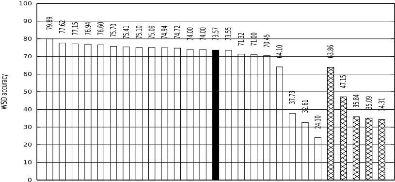
We note that re-sampling the training examples gives better WSD improvements than merely adjusting the posteriori probabilities output by the classifier. The number of training examples for a sense will affect the accuracy of the classifier trained for that sense. Thus, if one has a reliable estimate of the sense distribution, it might be more beneficial to resample the training examples. The results show that sampling a maximum of 500 examples per noun from the parallel texts according to the distribution estimated by the EM algorithm gives our best achievable WSD accuracy of 73.57% (72.21% + 1.36%). In the column EM sample of Table 2, we show the WSD accuracy resulting from sampling parallel text examples according to the EM estimated sense distribution, with different maximum number of examples per noun (i.e., this column is obtained by adding the figures from the columns L and EM-L sample).
4.2 Comparison with SE2 Systems
We compare our WSD accuracy achieved with the SENSEVAL-2 English lexical sample task participating systems. We performed sense lumping on the publicly available predictions of the SENSEVAL-2 participating systems. The WSD accuracy of each system is then calculated over the set of 22 nouns. In the SENSEVAL-2 English lexical sample task, there were 21 supervised and 5 1 unsupervised systems. Figure 1 shows the relative ranking of our system (which we named Parallel-EM) against the various SE2 systems.
We note that our system achieved better performance than all the unsupervised systems, and would have ranked at the 64% percentile among the list of 22 (including ours) supervised systems.
5 Discussion
The score of 73.57% achieved by Parallel-EM is competitive, considering that the SE2 supervised systems are trained with the manually annotated official data, while our system was trained with examples automatically extracted from parallel texts. Moreover, the following factors will also have to be considered.
Official Training Data has Similar Sense Distribution as Test Data
This is an advantage that the participating SENSEVAL-2 supervised systems enjoy. Note that the results in Table 2 show that if we sample according to the true distribution with a maximum of 500 examples per noun, we could achieve a score of 74.61%.
1 There were 4 systems from IIT (2 were resubmissions), but system answers were only available for 2 of them.
Some Official Training and Test Examples are from the Same Document
Our prior work [Ng et al., 2003] highlighted the fact that many of the official SENSEVAL-2 training and test examples are extracted from the same document, and that this has inflated the accuracy figures achieved by SENSEVAL-2 participating systems.
To investigate this effect, we trained our WSD classifier using the official training examples. When evaluated on the official test examples, a WSD accuracy of 79.71% was achieved. Next, we followed the steps taken in [Ng et al., 2003]: We took the official training and test examples of each noun w and combined them together. The combined data is then randomly split into a new training and a new test set such that no training and test examples come from the same document. While performing the split, we ensured the sense distribution of the new training and test data sets followed those of the official data sets. A WSD classifier was then trained on this new training set, and evaluated on this new test set. 5 random trials were conducted, and our WSD classifier achieved an accuracy of 77.83% (a drop of 1.88% from 79.71%).
Lack of Parallel Training Examples for some Senses
A disadvantage faced by Parallel-EM is that, though the senses are lumped, we are still lacking training examples for 9.64% of the test data. We believe that with the steady increase in volume and variability of parallel corpora, this problemwill improve in the near future.
Domain Difference
Lastly, we note that 91% of the SENSEVAL-2 English lexical sample task test examples were drawn from BNC. This represents a domain difference with our parallel corpora, which is mainly a mix of legislative, law, and news articles. Examples from different domains will contain different information, thus presenting different classification cues to the learning algorithm.
6 Conclusion
Differences in sense distribution between the training and test sets will result in a loss of WSD accuracy. Addressing this issue is important, especially if one is to build WSD systems that are portable across different domains, of which the difference in sense distribution is an inherent issue. In this paper, we used two distribution estimation algorithms to provide estimates of the sense distribution in a new data set. When applied on the nouns of the SENSEVAL-2 English lexical sample task, we have shown that they are effective in improving WSD accuracy.
Acknowledgements
The first author is supported by a Singapore Millennium Foundation Scholarship (ref no. SMF-2004-1076). This research is also partially supported by a research grant R252000-125-112 from National University of Singapore Academic Research Fund.
@inproceedings{ijcai2005p202,
  title     = {Word Sense Disambiguation with Distribution Estimation},
  author    = {Chan, Yee Seng and Ng, Hwee Tou},
  booktitle = {Proceedings of the Nineteenth International Joint Conference on
               Artificial Intelligence, {IJCAI-05}},
  publisher = {International Joint Conferences on Artificial Intelligence},
  editor    = {Leslie Pack Kaelbling and Alessandro Saffiotti},
  pages     = {1010--1014},
  year      = {2005},
  url       = {https://ijcai.org/proceedings/2005/202},
}
TY - CPAPER TI - Word Sense Disambiguation with Distribution Estimation AU - Chan, Yee Seng AU - Ng, Hwee Tou T2 - Proceedings of the Nineteenth International Joint Conference on Artificial Intelligence, IJCAI-05 PB - International Joint Conferences on Artificial Intelligence PY - 2005 SP - 1010 EP - 1014 UR - https://ijcai.org/proceedings/2005/202 ER -Copied
Machine-readable versions of this paper, for tools and AI agents:





