
Dynamically Constructed Bayes Nets for Multi-Domain Sketch Understanding
Proceedings of the Nineteenth International Joint Conference on Artificial Intelligence. Pages 1407-1411.
© 2005 International Joint Conferences on Artificial Intelligence
Abstract
This paper presents a novel form of dynamically constructed Bayes net, developed for multi-domain sketch recognition. Our sketch recognition engine integrates shape information and domain knowledge to improve recognition accuracy across a variety of domains using an extendible, hierarchical approach. Our Bayes net framework integrates the influence of stroke data and domain-specific context in recognition, enabling our recognition engine to handle noisy input. We illustrate this behavior with qualitative and quantitative results in two domains: hand-drawn family trees and circuits.
- [Alvarado and Davis, 2004] C. Alvarado and R. Davis. SketchREAD: A multi-domain sketch recognition engine. In Proc. of UIST-04, 2004.
- [Alvarado, 2004] C. Alvarado. Multi-Domain Sketch Understand- ing. PhD thesis, MIT, 2004.
- [bnj, 2004] Bayesian network tools in java (bnj), 2004. http://bnj.sourceforge.net. Link
- [Boutilier et al., 1996] C. Boutilier, N. Friedman, M. Goldszmidt, and D. Koller. Context-specific independence in Bayesian net- works. In Proc. of UAI '96, 1996.
- [Futrelle and Nikolakis, 1995] R. P. Futrelle and N. Nikolakis. Effi- cient analysis of complex diagrams using constraint-based pars- ing. In ICDAR-95, pages 782-790, Montreal, Canada, 1995.
- [Getoor et al., 1999] L. Getoor, N. Friedman, D. Koller, and A. Pf- effer. Learning probabilistic relational models. In Proc. of IJCAI '99, pages 1300-1309, 1999. IJCAI
- [Glessner and Koller, 1995] S. Glessner and D. Koller. Construct- ing flexible dynamic belief networks from first-order proba- bilistinc knowledge bases. In Synbolic and Quantitatice Ap- proaches to Reasoning and Uncertainty, pages 217-226, 1995.
- [Haddawy, 1994] P. Haddawy. Generating bayesian networks from probability logic knowledge bases. In Proc. of UAI '94, 1994.
- [Hammond and Davis, 2003] T. Hammond and R. Davis. LAD- DER: A language to describe drawing, display, and editing in sketch recognition. Proc. of IJCAI '03, 2003.
- [Hammond and Davis, 2004] T. Hammond and R. Davis. Automat- ically transforming symbolic shape descriptions for use in sketch recognition. Proc. of AAAI '04, 2004.
- [Jensen et al., 1990] F. V. Jensen, S. L. Lauritzen, and K. G. Ole- sen. Bayesian updating in causal probabilistic networks by local computations. Computational Statistics Quarterly, 4, 1990.
- [Kara and Stahovich, 2004] L. B. Kara and T. F. Stahovich. Hier- archical parsing and recognition of hand-sketched diagrams. In Proc. of UIST '04, 2004.
- [Koller and Pfeffer, 1997] D. Koller and A. Pfeffer. Object-oriented bayesian networks. In Proc. of UAI '97, 1997.
- [Laskey and Mahoney, 1997] K. B. Laskey and S. M. Mahoney. Network fragments: Representing knowledge for constructing probabilistic models. In Proc. of UAI '97, 1997.
- [Oltmans et al., 2004] M. Oltmans, C. Alvarado, and R. Davis. Etcha sketches: Lessons learned from collecting sketch data. In Making Pen-Based Interaction Intelligent and Natural. AAAI Fall Symposium, 2004.
- [Pfeffer et al., 1999] A. Pfeffer, D. Koller, B. Milch, and K. Takusagawa. SPOOK: A system for probabilistic object- oriented knowledge representation. In Proc. of UAI '99, 1999.
- [Weiss, 1997] Y. Weiss. Belief propagation and revision in net- works with loops. Technical report, MIT, November 1997.
- [Wu et al., 1999] L. Wu, S. L. Oviatt, and P. R. Cohen. Multimodal integration-a statistical view. IEEE Transaction on Multimedia, 1(4):334-341, December 1999.
References were extracted automatically from the PDF and may contain errors.
Full text extracted automatically from the PDF; figures, tables and equations may differ. The PDF is the version of record.
1 Introduction
There is a gap between how people naturally express ideas and the ability of computers to use that information. For example, while sketching provides a natural way to record design ideas in many domains, sketches are, unavoidably, static pictures. Computer aided design tools, on the other hand, offer powerful capabilities, but require designers to interact through buttons and menus. The hardware to draw on the computer exists; the missing element is the computer's ability to interpret hand-drawn symbols in a domain. To address this problem, we are constructing a general sketch recognition architecture applicable to a number of domains, and capable of parsing freely-drawn strokes in real time and interpreting them as depicting objects in the domain of interest.
Sketch recognition involves two related subproblems: stroke segmentation and symbol recognition. Segmentation determines which strokes should be grouped to form a single symbol. Symbol recognition determines what symbol a given set of strokes represents.
The difficulty of doing segmentation and recognition simultaneously has led previous approaches to place constraints on the user's drawing style, or focus on tasks where assumptions can greatly reduce segmentation complexity. For example, the multimodal approach in [Wu et al., 1999] assumes that each symbol will be drawn independently, and that the user will often say the name of the symbol when drawing it. The approach in [Kara and Stahovich, 2004] assumes that the diagram (a feedback control system) consists of shapes linked by arrows, which is not true in other domains.
∗Currently at Harvey Mudd College, Claremont, CA, 91711
† This work was funded by the MIT iCampus project supported by Microsoft and MIT Project Oxygen.
While these systems have proven useful for their respective tasks, we aimed to create a more general system, independent of drawing assumptions in any one domain. Our system is designed, instead, to be applied to a number of symbolic domains by giving it descriptions of shapes and commonly occurring combinations of shapes. We use these descriptions in a three-stage, constraint-based approach to recognition. Our system first relies on a rough processing of the user's strokes to generate a number of interpretation hypotheses. In the second stage, the system uses a novel form of dynamically constructed Bayes net to determine how well each hypothesis fits the data. In the third stage, it uses this evaluation to guide further hypothesis generation. This paper focuses specifically on the second stage, exploring hypothesis evaluation; the other two stages are described in [Alvarado, 2004].
Using Bayes nets for hypothesis evaluation offers two advantages over previous constraint-based recognition approaches (e.g., [Futrelle and Nikolakis, 1995; Hammond and Davis, 2004]). First, our system can interpret drawings as they develop, identifying shapes before they are complete. Second, the system's belief in a hypothesis can be influenced by both the strokes and the context in which the shape appears, allowing the system to cope with noise in the drawing.
We constructed a sketch recognition engine and used it in two domains: family tree diagrams and circuit diagrams. We show that the Bayes net successfully allows domain-specific context to help the system overcome noise in the stroke data, reducing interpretation errors compared to a baseline system.
2 Dynamically Constructed Graphical Models
While time-based graphical models (e.g., Dynamic Bayes Nets) have been widely used, they are not suitable for sketch understanding, for two reasons. First, we must model shapes based on two-dimensional constraints (e.g., touches) rather than on temporal constraints (i.e., follows). Second, our models cannot simply unroll in time as data arrives: we cannot necessarily predict the order in which the user will draw the strokes, and things drawn previously can be changed.
While it is not difficult to use Bayes nets to model spatial relationships, static Bayes nets are not suitable for our task
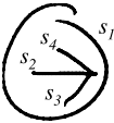
Primitive hypotheses
E 1 = ellipse-fit(s 1 )
L 1 = line-fit(s 2 )
L 2 = line-fit(s 3 )
L 3 = line-fit(s 4 )
Arrow hypothesis A 1 Subshapes:
line hypotheses L 1 , L 2 , L 3
Constraints:
C 2 = (coincident line-fit(s 2 ).p1 line-fit(s 3 ).p1)
C 3 = (coincident line-fit(s 2 ).p1 line-fit(s 4 ).p1)
C 4 = (equalLength line-fit(s 3 ) line-fit(s 4 ))
C 5 = (shorter line-fit(s 3 ) line-fit(s 2 ))
C 6 = (acuteAngle line-fit(s 2 ), line-fit(s 3 ))
C 7 = (acuteAngle line-fit(s 2 ), line-fit(s 4 ))
CS hypothesis CS 1
Subshapes:
arrow hypothesis A 1 , ellipse hypothesis E 1
Constraints:
C 1 = (contains ellipse-fit(s 1 ) shape-fit(s 2 ,s 3 ,s 4 ))
Figure 1: A single current source hypothesis (CS1) and associated lower-level hypotheses.
because we cannot predict a priori the number of strokes or symbols the user will draw. For sketch recognition, as in related dynamic tasks, models to reason about specific problem instances (e.g., a particular sketch) must be dynamically constructed in response the input. This problem is known as the task of knowledge-based model construction (KBMC).
Early approaches to KBMC focused on generating Bayes nets from probabilistic knowledge bases [Glessner and Koller, 1995; Haddawy, 1994]. A recently proposed representation uses generic template knowledge directly as Bayes net fragments that can be instantiated and linked together at run-time [Laskey and Mahoney, 1997]. Finally, Koller et al. have developed a number of object-oriented frameworks [Koller and Pfeffer, 1997; Pfeffer et al., 1999; Getoor et al., 1999]. These models represent knowledge in terms of relationships among objects and can be instantiated dynamically in response to the number of objects in a particular situation.
Although these frameworks are powerful, they are not directly suitable for sketch recognition. First, because of the size of the networks we encounter, it is sometimes desirable to generate only part of a complete network, or to prune nodes from the network. In reasoning about nodes in the network, we must account for the fact that the network may not be fully generated or relevant information may have been pruned from it (see [Alvarado, 2004] for details). Second, these previous models have been optimized for responding to specific queries about a single node in the network. In contrast, our model must provide probabilities for a full set of possible interpretations of the user's strokes.
3 Network Structure
Our Bayes net model is built around hierarchical descriptions of shapes in a domain, described in a language called LADDER [Hammond and Davis, 2003]. The basic unit in this language is a shape, which we use to mean a pattern recognizable in a given domain. Shapes may be compound, i.e., composed of subshapes fit together according to constraints. These subshapes also may be compound, but all shapes must be non-recursive. A shape that cannot be decomposed into subshapes (e.g., a line), is called a primitive shape. Primitive shapes may have named subcomponents that can be used when describing other shapes, e.g., the endpoints of a line, "p1" and "p2", used in Figure 1.
We refer to each shape description as a template with one slot for each subpart. A shape hypothesis is a template with an associated mapping between slots and strokes, generated during the recognition process. Similarly, a constraint hypothesis is a proposed constraint on one or more of the user's strokes. A partial hypothesis is a hypothesis in which one or more slots are not bound to strokes.
To introduce our Bayes net model, we begin by considering how to model a current source hypothesis (CS1) for the stokes in Figure 1. A current source is a compound shape, soCS1 involves two lower-level shape hypotheses-E1, an ellipse hypothesis for stroke s1; and A1, an arrow hypothesis involving strokes s2, s3 and s4-and one constraint hypothesis-C1, indicating that an ellipse fit for stroke s1 contains strokes s2, s3, and s4. A1 is also compound and is further broken down into three line hypotheses (L1, L2 and L3) and six constraint hypotheses (C2↪ ▷▷▷↪C7) according to the description of an arrow. Thus, determining the strength of hypothesis CS1 can be transformed into the problem of determining the strength of a number of lower-level shape and constraint hypotheses.
The Bayes net used to evaluate CS1 is shown in Figure 2. There is one node in the network for each hypothesis; each node represents a boolean random variable that is true if the corresponding hypothesis is correct. The probability of each hypothesis is influenced both through its children by stroke data and through its parents by the context in which it appears, allowing the system to handle noise in the drawing.
The nodes labeled O1↪ ▷▷▷↪O11 represent measurements of the stroke data that correspond to the constraint or shape to which they are linked. The variables corresponding to these nodes have positive real numbered values that we discretize in our implementation 1 . For example, the variable O2 is a measurement of the squared error between the stroke s1 and the best fit ellipse to that stroke. Its raw value (later discretized) ranges from 0 to the maximum possible error between any stroke and an ellipse fit to that stroke. The boxes labeled s1↪ ▷▷▷↪s4 are not part of the Bayes net but serve to indicate the stroke or strokes from which each measurement, Oi, is taken (e.g., O2 is measured from s1). P(CS1 = t|ev) (or simply P(CS1|ev)) 2 , where ev is the evidence observed from the user's strokes, represents the probability that the hypothesis CS1 is correct.
The direction of the links may seem counterintuitive, but there are two important reasons why the links are directed from higher-level shapes to lower-level shapes instead of the opposite direction. First, whether a higher-level hypothesis is true directly influences whether a lower-level hypothesis is true. For example, if the arrow hypothesis A1 is true, then it is extremely likely that all three line hypotheses, L1↪L2↪L3, are also true. Second, this representation allows us to model lower-level hypothesis as conditionally independent given their parents, which reduces the complexity of the data needed to construct the network.
1 The BN software we used did not support continuous variables.
2 Throughout this paper, t means true, and f means false.
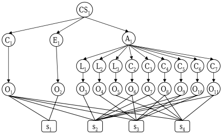
Each shape description constrains its subshapes only relative to one another. For example, an arrow may be made from any three lines that satisfy the necessary constraints. Based on this observation, our representation models a symbol's subshapes separately from the constraints between them. For example, node L2 represents the hypothesis that stroke s3 is a line. Its value will be true if the user intended for s3 to be a line, any line regardless of its position, size or orientation. C4 separately represents the hypothesis that the line fit to s3 and the line fit to s4 are the same length.
The conditional independence between shapes and constraints might seem a bit strange at first. For example, whether or not two lines are the same length seems to depend on the fact that they are lines. However, observation nodes for constraints are calculated in such a way that their value is not dependent on the true interpretation for a stroke. For example, when calculating whether or not two lines are the same length, we first fit lines to the strokes (regardless of whether or not they actually look like lines), then measure their length. How well these lines fit the original strokes is not considered in this calculation.
The fact that there is no edge between the constraint nodes and the shapes they constrain has an important implication for using this model to perform recognition: There is no guarantee in this Bayes net that the constraints will be measured between the correct subshapes because the model allows subshapes and constraints to be detected independently. For example, we want C4 in Figure 2 to indicate that L2 and L3 (the two lines in the head of an arrow) are the same length, not simply that any two lines are the same length. To satisfy this requirement, the systemmust ensure that O8 is measured from the same strokes that O4 and O5 were measured from. We use a separate mechanism to ensure that only legal bindings are created between strokes and observation nodes.
The way we model shape and constraint information has two important advantages for recognition. First, this Bayes net model can be applied to recognize a shape in any size, position and orientation. CS1 represents the hypothesis that s1↪ ▷▷▷↪s4 form a current source symbol, but the exact position, orientation and size of that symbol is determined directly from the stroke data 3 .
Second, the system can model competing higher-level interpretations for lower-level shapes. For example, the system may consider a stroke to be a line that is in turn part of either an arrow or a quadrilateral. Because the line hypothesis does not include any higher-level shape-specific constraint information, both an arrow hypothesis node and a quadrilateral hypothesis node can point to this same line hypothesis node. These two hypotheses then become alternate, competing explanations for the line hypothesis. We further discuss how hypotheses are combined below.
4 Recognizing a Complete Sketch
To recognize a complete sketch, we create a Bayes net similar to the one above for each shape. We call each of these Bayes nets a shape fragment because they can be combined to create a complete Bayes net for evaluating the whole sketch.
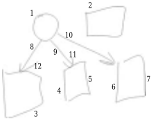
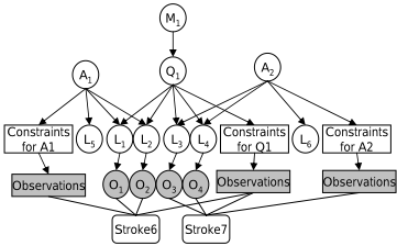
Given a set of hypotheses for the user's strokes (hypothesis generation is described in [Alvarado and Davis, 2004] and [Alvarado, 2004]), the system instantiates the corresponding shape fragments and links them together to form a complete Bayes net, called the interpretation network. To illustrate this process, consider a piece of a network generated in response to Strokes 6 and 7 in the example of Figure 3. Figure 4 shows the part of the Bayes net representing the hypotheses that the system generated for these strokes. Low level processing recognizes Strokes 6 and 7 as L-shaped polylines and breaks each into two individual lines (L1▷▷▷L4) that meet.
4.1 Linking Shape Fragments
When Bayes net fragments are linked during recognition, each node Hn may have several parents, S1 ▷ ▷ ▷ Sm, where each parent represents a possible higher-level interpretation for Hn. We use a noisy-OR function to combine the influences of all the parents of Hn to produce the complete conditional probability table (CPT) for P(Hn|S1↪ ▷ ▷ ▷ ↪Sm). The noisy-OR function models the assumption that each parent can independently cause the child to be observed. For example, a single stroke might be part of a quadrilateral or an arrow, but both interpretations would favor that interpretation of the stroke as a line. We set P(Hn = f |Sj = t) = 0 for all parents Sj in which Hn is a required subshape or constraint, and we set P(Hn = f |Sk = t) = 0▷5 for all parents Sk in which Hn is an optional subshape or constraint. A consequence of these values is that Sj = t ⇒P(Hn|S1↪ ▷ ▷ ▷ ↪Sm) =1 for any Sj in which Hn is required, which is exactly what we intended.
3 Orientation-dependent symbols (e.g., a downward-facing arrow) can be recognized by including orientation-dependent constraints in their descriptions (e.g., vertical, below).
We experimented with a noisy-XOR construct, implemented using a "gate node" similar to that described in [Boutilier et al., 1996], but found that noisy-OR semantics were simpler and in fact produced better results. In effect, a noisy-OR node in a Bayes net with low prior probabilities behaves as a non-aggressive XOR. The fact that one parent is true does not actively prohibit the other parents from being true, but it causes their probabilities to tend back to their prior values because of the "explaining away" phenomenon.
4.2 Signal Level Noise
The bottom layer of the network deals with signal level noise by modeling the differences between the user's intentions and the strokes that she draws. For example, even if the user intends to draw L1, her stroke likely will not match L1 exactly, so the model must account for this variation. Consider P(O1|L1 = t) (recall that O1 is a discretized continuous valued variable). If the user always drew perfect lines, this distribution would be 1 when O1 = 0 (i.e., the error is 0), and 0 otherwise. However, most people do not draw perfect lines (due to inaccurate pen and muscle movements), and this distribution allows for this error. It should be high when O1 is close to zero, and fall off as O1 gets larger. The wider the distribution, the more error the system will tolerate, but the less information a perfect line will provide.
The other distribution needed is P(O1|L1 = f ) which is the probability distribution over line error given that the user did not intend to draw an line. This distribution should be close to uniform, with a dip around 0, indicating that if the user specifically does not intend to draw an line, she might draw any other shape, but probably won't draw anything that resembles an line. Details about how we determined the conditional probability distributions between primitive shapes and constraints and their corresponding observation nodes are given elsewhere [Alvarado, 2004].
4.3 Missing Strokes
A1 is a partial hypothesis-it represents the hypothesis that L1 and L2 (from Stroke 6) are part of an arrow whose other line has not yet been drawn. Line nodes representing lines that have not been drawn (e.g., L5) are not linked to observation nodes because there is no stoke from which to measure these observations. We refer to these nodes (and their corresponding hypotheses) as virtual.
The fact that partial hypotheses have probabilities allows the system to assess the likelihood of incomplete interpretations based on the evidence it has seen so far. In fact, even virtual nodes have probabilities, corresponding to the probability that the user (eventually) intends to draw these shapes but either has not yet drawn this part of the diagram or the correct low-level hypotheses have not yet been proposed (because of low-level recognition errors). A partial hypothesis with a high probability cues the system to examine the sketch for possible missed low-level interpretations during the hypothesis generation step.
5 Implementation and Bayesian Inference
Our system updates the structure of the Bayes net in response to each stroke the user draws, using an off-the-shelf, open source Bayes net package for Java called BNJ [bnj, 2004].
Generating and modifying the BNJ networks can be time consuming due to the exponential size of the CPTs between the nodes. We use two techniques to improve performance. First, networks are generated only when the system needs to evaluate the likelihood of a hypothesis. This on-demand construction is more efficient than continuously updating the network, because batch construction of the CPTs is often more efficient than incremental construction. Second, the system modifies only the portion of the network that has changed between strokes, rather than creating it from scratch every time.
We experimented with several inference methods and found that loopy belief propagation (loopy BP) [Weiss, 1997] was the most successful 4 . On our data, loopy BP almost always converged (messages initialized to 1, run until node values stable within 0.001). We further limited the algorithm's running time in two ways. First, we terminated the algorithm after 60 seconds if it had not yet converged. Second, we allowed each node to have no more than 8 parents (i.e., only 8 higher-level hypotheses could be considered for a single hypothesis), ensuring a limit on the complexity of the graphs produced. These restrictions had little impact on recognition performance in the family tree domain, but for complex domains such as circuit diagrams, more efficient inference algorithms or graph simplification techniques are needed to improve recognition results.
6 Application and Results
We applied our implemented system to two non-trivial domains-family trees and circuits-and found that it is capable of recognizing sketches in both domains without reprogramming. Qualitative and quantitative evaluation of our system illustrates its strengths over previous approaches and suggests some extensions.
4 Junction Tree [Jensen et al., 1990] was often too slow and Gibb's Sampling did not produce meaningful results.
Applying our system to a particular domain involves two steps: specifying the structural descriptions for the shapes in the domain, and specifying the prior probabilities for toplevel shapes and domain patterns, i.e., those that will not have parents in the Bayes net. For each domain, we wrote a description for each shape and pattern in that domain. We handestimated priors for each domain pattern and top level shape based on our intuition about the relative prevalence of each shape. For example, in family-tree diagrams, we estimated that marriages were much more likely than partnerships, and set P[Mar] = 0▷1 and P[Part ] = 0▷001. These priors represent the probability that a group of strokes chosen at random from the page will represent the given shape and, in most cases, should be relatively low. Although setting priors by hand can be tedious, we found through experimentation that the system's recognition performance was relatively insensitive to the exact values of these priors. For example, in the circuit diagrams, increasing all the priors by an order of magnitude did not affect recognition performance; what matters instead is the relative values of the prior probabilities.
Our system is capable of recognizing simple sketches nearly perfectly in both the family-tree and circuit domains. We also tested its performance on more complex, real-world data. As there is no standard test corpus for sketch recognition, we collected our own sketches and have made them available online to encourage others to compare their results with those presented here [Oltmans et al., 2004]. In total, we tested our system on 10 family tree sketches and 80 circuit diagram sketches, with between 23 and 110 strokes each.
6.1 Qualitative Results
Qualitative analysis reveals that the Bayes net mechanism successfully aggregates information from stroke data and context, resolves inherent ambiguities in the drawing, and updates its weighting of the various existing hypotheses as new strokes are drawn. We show through an example that the Bayes net scores hypotheses correctly in several respects: it prefers to group subshapes into the fewest number of interpretations, it allows competing interpretations to influence one another, it updates interpretation strengths in response to new stroke data, and it allows both stroke data and context to influence interpretation strength.
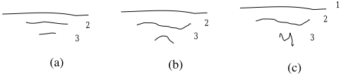
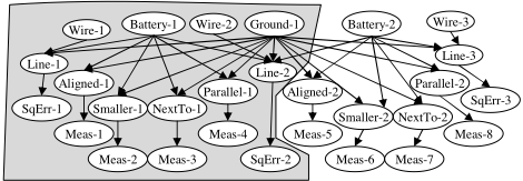
To illustrate the points above, we consider in detail how the system responds as the user draws the three sets of strokes in Figure 5 (a ground symbol). To simplify the example, we consider a reduced circuit domain in which users draw only wires, resistors, ground symbols and batteries. Figure 6 shows the Bayes nets produced in response to the user's first two and first three strokes. After the first two strokes, the network contains only the nodes in the shaded area; after three strokes it contains all nodes shown. Continuous variables corresponding to observation nodes were discretized into three values: 0 (low error: stroke data strongly supports the shape or constraint), 1 (medium error: stroke data weakly supports the shape or constraint), and 2 (high error: stroke data does not support the shape or constraint).
| Name | P[Shape|stroke data] | |||||
|---|---|---|---|---|---|---|
| after 2 strokes | after 3 strokes | |||||
| (a) | (b) | (c) | (a) | (b) | (c) | |
| Wire-1 | 0.4 | 0.41 | 0.41 | 0.4 | 0.4 | 0.42 |
| Wire-2 | 0.4 | 0.38 | 0.38 | 0.4 | 0.4 | 0.38 |
| Wire-3 | N/A | N/A | N/A | 0.4 | 0.4 | 0.1 |
| Battery-1 | 0.51 | 0.51 | 0.51 | 0.09 | 0.1 | 0.91 |
| Battery-2 | N/A | N/A | N/A | 0.09 | 0.1 | 0.0 |
| Ground-1 | 0.51 | 0.51 | 0.51 | 0.95 | 0.94 | 0.03 |
Posterior probabilities are given in Table 1. For the relatively clean ground symbol (Figure 5(a)), the stroke data strongly supports all the shapes and constraints, so all shaded nodes in Figure 6 have value 0. After the first two strokes, the battery symbol and the ground symbol have equal weight, which may seem counterintuitive: after two strokes the user has drawn what appears to be a complete battery, but has drawn only a piece of the ground symbol. Recall, however, that the Bayes net models not what has been drawn, but what the user intends to draw. After two strokes, it is equally likely that the user is in the process of drawing a ground symbol. After the third stroke, the ground symbol's probability increases because there is more evidence to support it, while the battery's probability decreases. The fact that the ground symbol is preferred over the battery illustrates that the system prefers interpretations that result in fewer symbols (Okham's razor). Interpretations that involve more of the user's strokes have more support and get a higher score in the Bayes net. The fact that the battery symbol gets weaker as the ground symbol gets stronger results from the "explaining away" behavior in this Bayes net configuration: each of the low-level components (the lines and the constraints) are effectively "explained" by the existence of the ground symbol, so the battery is no longer needed to explain their presence.
Another useful property of our approach is that a small amount of noise in the data is counteracted by the context provided by higher-level shapes. The slightly noisy second and third strokes in Figure 5(b) cause the values of SqErr2 and SqErr-3 to be 1 instead of 0 (all other shaded node values remain 0). Despite this noise, after three strokes the posterior probability of the ground symbol interpretation is still high (0.94), because Line-1 and all of the constraints are still strongly supported by the data. In addition, the probabilities for Line-2 and Line-3 are high (both 1.0, not shown in Table 1), indicating that the context provided by the ground symbol provides support for the line interpretations even when the evidence from the data is not as strong.
On the other hand, if the data is too messy, it causes the probability of the higher-level interpretations to decrease. The sketch in Figure 5(c) causes the value of SqErr-2 to be 1, and SqErr-3 to be 2, and results in a low posterior probability for Ground-1 (0.03) and a high posterior for Battery-1 (0.91), because the hypothesis Line-3 is contradicted by the user's third stroke. For now, the third stroke remains uninterpreted.
6.2 Quantitative Results
We ran our system on all of the sketches we collected and compared its performance to a baseline constraint-based recognition system that used a fixed threshold for detecting shapes and constraints and did not reinterpret low-level shapes. We measured recognition performance by determining the number of objects identified correctly in each sketch. Our system significantly outperformed the baseline system (p≪0▷001), correctly recognizing 77% (F=0.83) of the shapes in the family tree diagrams and 62% (F=0.65) of the shapes in the circuit diagrams, while the baseline system correctly recognized 50% (F=0.63) and 54% (F=0.57).
While not yet real time, in general our system's processing time scaled well as the number of strokes increased. However, it occasionally ran for a long period. The system had particular trouble with areas of the sketch that involved many strokes drawn close together in time and space and with domains that involve more complicated or overlapping symbols. This increase in processing time was due almost entirely to increase in Bayes net complexity.
We believe we can speed up loopy BP based on the observation that it repeatedly sends messages between the nodes until each node has reached a stable value. When a stroke is added, our system resets all messages to 1, essentially erasing the work done the last time inference was performed, even though most of the graph is unchanged. The algorithm should instead begin with the messages that remain at the end of the previous inference step.
7 Conclusion
We have described a model for dynamically constructing Bayes nets to represent varying hypotheses for the user's strokes. Our model, specifically developed for the task of recognition, allows both stroke data and contextual data to influence the probability of an interpretation for the user's strokes. Using noisy-OR, multiple potential higher-level interpretations mutually influence each other's probabilities within the Bayes net. The net result is a sketch recognition approach that brings us a significant step closer to sketching as a natural and powerful interface.
@inproceedings{ijcai2005p198,
  title     = {Dynamically Constructed Bayes Nets for Multi-Domain Sketch Understanding},
  author    = {Alvarado, Christine and Davis, Randall},
  booktitle = {Proceedings of the Nineteenth International Joint Conference on
               Artificial Intelligence, {IJCAI-05}},
  publisher = {International Joint Conferences on Artificial Intelligence},
  editor    = {Leslie Pack Kaelbling and Alessandro Saffiotti},
  pages     = {1407--1411},
  year      = {2005},
  url       = {https://ijcai.org/proceedings/2005/198},
}
TY - CPAPER TI - Dynamically Constructed Bayes Nets for Multi-Domain Sketch Understanding AU - Alvarado, Christine AU - Davis, Randall T2 - Proceedings of the Nineteenth International Joint Conference on Artificial Intelligence, IJCAI-05 PB - International Joint Conferences on Artificial Intelligence PY - 2005 SP - 1407 EP - 1411 UR - https://ijcai.org/proceedings/2005/198 ER -Copied
Machine-readable versions of this paper, for tools and AI agents:





