
Generalization Bounds for Weighted Binary Classification with Applications to Statistical Verification
Proceedings of the Nineteenth International Joint Conference on Artificial Intelligence. Pages 722-726.
© 2005 International Joint Conferences on Artificial Intelligence
Abstract
We describe an approach to statistically verifying complex controllers. This approach is based on deriving practical Vapnik-Chervonenkis-style (VC) generalization bounds for binary classifiers with weighted loss. An important case is deriving bounds on the probability of false positive. We show how existing methods to derive bounds on classification error can be extended to derive similar bounds on the probability of false positive, as well as bounds in a decision-theoretic setting that allows tradeoffs between false negatives and false positives. We describe experiments using these bounds in statistically verifying computational properties of an iterative controller for an Organic Air Vehicle (OAV).
- P. L. Bartlett, S. Boucheron, and G. Lugosi. Model selection and error estimation. Mach. Learn., 48(1-3):85-113, 2002.
- P.L. Bartlett, O. Bousquet, and S. Mendelson. Local Rademacher complexities. Annals of Statistics, 2005. To appear.
- A. Blumer, A. Ehrenfeucht, D. Haussler, and M. K. Warmuth. Learnability and the Vapnik-Chervonenkis dimension. J. ACM, 36(4):929-965, 1989.
- O. Bousquet. A Bennett concentration inequality and its application to suprema of empirical processes. C. R. Acad. Sci. Paris, Ser. I, 334:495-500, 2002.
- R. Dudley. Uniform Central Limit Theorems. Cambridge University Press, Cambridge, MA, 1999.
- M.R. Elgersma and B.G. Morton. Nonlinear six-degree-of-freedom aircraft trim. Journal of Guidance, Control, and Dynamics, 23(2):305-311, 2000.
- D. Haussler. Sphere packing numbers for subsets of Boolean n- cube with bounded Vapnik-Chervonenkis dimension. Journal of Combinatorial Theory (A), 69:217-232, 1995.
- V. Koltchinskii and D. Panchenko. Rademacher processes and bounding the risk of function learning. High Dimensional Prob- ability II, 47:443-459, 2000.
- V. Koltchinskii. Rademacher penalties and structural risk minimiza- tion. IEEE Transactions on Information Theory, 47(5):1902- 1914, July 2001.
- P. Massart. Some applications of concentration inequalities to statis- tics. Annales de la Faculté des Sciences de Toulouse, IX(2):245- 303, 2000.
- C. McDiarmid. Concentration. In M. Habib, C. McDiarmid, J. Ramirez-Alfonsin, and B. Reed, editors, Probabilistic method for algorithmic discrete mathematics, pages 195-248. Springer- Verlag, New York, 1997.
- D. Panchenko. Some extensions of an inequality of Vapnik and Chervonenkis. Electronic Communications in Probability, 7:55- 65, 2002.
- N. Sauer. On the density of families of sets. Journal of Combinato- rial Theory, 13:145-147, 1972.
- John Shawe-Taylor, Martin Anthony, and N. L. Biggs. Bounding sample size with the Vapnik-Chervonenkis dimension. Discrete Appl. Math., 42(1):65-73, 1993.
- M. Talagrand. Sharper bounds for gaussian and empirical processes. Annals of Probability, 22:20-76, 1994.
- M. Talagrand. New concentration inequalities for product spaces. Inventiones Mathematicae, 126(3):505-563, 1996.
- P. Turney. Types of cost in inductive concept learning. In Workshop on Cost-Sensitive Learning at the Seventeenth International Con- ference on Machine Learning, pages 15-21, Stanford University, California, 2000.
- V. Vapnik and A. Chervonenkis. On the uniform convergence of relative frequencies of events to their probabilities. Theory of Probability and Its Applications, 16:264-280, 1971.
- V. Vapnik. The Nature of Statistical Learning Theory. Springer, second edition, 2000.
- M. Vidyasagar. Learning and Generalization, with Applications to Neural Networks. Springer, second edition, 2003.
References were extracted automatically from the PDF and may contain errors.
Full text extracted automatically from the PDF; figures, tables and equations may differ. The PDF is the version of record.
1 Introduction
The computational requirements for high-performance complex control algorithms can vary considerably. The variation arises because the computation depends on a number of factors such as the sensed/estimated state of the system under control, environmental disturbances, and the operational mode of the system. Furthermore, the variation in general can not be determined analytically. In hard real-time systems where the computation must complete in time for a command to be issued to the actuator at the next sample instant, these uncertainties pose a significant challenge. This is the reason that PID (Proportional-Integral-Derivative) controllers, with their deterministic execution time, are still the preferred choice in many applications despite their lesser performance.
In order to bring practical acceptance to high-performance complex control algorithms, we propose a compromise that makes use of both types of controller algorithms. Highperformance algorithms will be used within a safe operational envelope (SOE) where they are guaranteed to complete within the allocated time. Outside of the SOE, lower performance and computationally simpler algorithms will be used. The SOE is determined based on simulation data, and hence is only safe with some statistical guarantees.
The problem of identifying the SOE is a binary classification problem where a false negative merely means a conservative use of a low performance controller and a false positive may have drastic consequences such as loss of the vehicle. Thus we would like to obtain an SOE that has some statistical guarantee that it is indeed safe, i.e., a classifier with provably small probability of false positive. This however is not the only criterion, for otherwise the trivial classifier that classifies everything as negative, namely the current state of the art, would be the top candidate. Instead, the goal is to push the boundaries of the SOE as far as possible while keeping a cap on the probability of false positive.

As an example, let us consider the computational property of a high-performance controller for an OAV (Figure 1). The OAV has a ducted fan propulsion unit, with control provided by movable vanes in the propwash. The vanes are situated in the propulsion airflow and consequently the interactions between the propulsion and the control surfaces are highly non-linear. The trim calculation for the OAV is an iterative algorithm whose computational time depends on several factors [Elgersma and Morton, 2000]. We are interested in conditions under which this calculation can be reliably used.
Our approach is based on statistical learning theory (SLT). Specifically, we derive statistical guarantees for SOEs using Vapnik-Chervonenkis-style generalization bounds for classification problems with weighted loss, of which the classification problem with false positive loss is a special case. We are interested practical bounds-bounds that are asymptotically competitive and have small pre-constants. While the SLT literature contains a vast collection of VC-style bounds, the majority of these bounds are stated and proved only for the probability of misclassification and only a few are directly applicable to our problem. Furthermore, SLT bounds are often derived with little emphasis on obtaining optimal pre-constants. In addition to the emphasis on finding small pre-constants, our analysis has two unique aspects. First, we assume that it is possible to achieve small empirical loss (which is true for the case of false positive loss). Second, our analysis is upper-tail-oriented, as we are only interested in deriving upper bounds for the expected loss.
2 Preliminaries
Notations: We use the symbols P, E, and V to denote the probability, expectation, and variance, respectively. σ = {σi}ni=1 denotes a Rademacher sequence-a sequence of independent, symmetric -1/1-valued random variables.
Let X and Y be non-empty sets and Z = X × Y . A pair of (x, y) ∈ X × Y is denoted as z. Let (Z, µ) be a fixed probability measure. A training set is a finite sample Sn = {zi}ni=1 = {(xi, yi)}ni=1 ∈ Z n drawn independently according to µ. The probability and expectation with respect to Sn are written as Pn and En. A hypothesis space is a set H of functions from X to Y . A loss function is a function l : Y × Y → R. The loss of a hypothesis h ∈ H on z is l(h, z) = l(h(x), y). The expected loss of h is l(h) = El(h, z). The empirical loss of h on the training set Sn is ln(h) = l(h, Sn) = 1n ∑ni=1 l(h, zi). We assume that all loss functions have range [0, 1]. When Y is finite, we have a classification problem. When |Y | = 2, the classification is binary, and let Y = {-1, 1}. Here we only deal with binary classification.
If we assume that correct classifications incur zero loss, i.e. l(-1, -1) = l(1, 1) = 0, then what emerges is a loss function that we refer to as weighted classification error, defined as:
Here ρ is a number between 0 and 1. The idea is that false positives (bad errors) are more costly than false negatives (good errors). When ρ = 1, i.e. when no difference is made between the two types of errors, the loss is called the misclassification error. When ρ = 0, l(0) (h) is the probability of the classifier h making a false positive error.
Given a training set Sn, a hypothesis h ∈ H, and a loss function l, how can we bound the expected loss l(h)? Statistical learning theory (SLT) provides a probabilistic answer to this question. A typical SLT result of the form Pn(l(h) > ǫ) < δ or, succinctly, l(h) <δ ǫ provides an upper bound ǫ on l(h) with confidence at least 1 - δ, where ǫ and δ are positive, reasonably small numbers. The upper bound ǫ typically depends on δ, the sample size n, the empirical loss ln(h), and a complexity measure of the hypothesis space H. The most important complexity measure in SLT is VC dimension. Let C ⊆ 2X be a set of subsets of X. Note that H, as a set of binary classifiers on X, is an example of such sets. For any A ⊆ X, define C ∩ A = {C ∩ A : C ∈ C}. The growth function of C is defined as
Clearly, ∆k(C) ≤ 2k . The VC Dimension of C is defined as
Let d = d(H). We assume that d < ∞.
Theorem 2.1. [Vapnik, 2000, Equations 3.26]
The bound (2.1) is obtained by applying a very general result of Vapnik to the special setting of learning binary classifiers with a specific loss function l(ρ) . It is thus natural to ask if this bound can be improved. While many SLT results have been obtained that address this issue, the majority of are formulated and proved for l = l(1) only. One of the goals of this paper is to examine if these results can be extended to the loss functions l(ρ) , ρ ∈ [0, 1). It turns out that these results fall into two categories: those that are applicable for all ρ ∈ [0, 1], and those that are applicable for ρ = 0, 1 only.
We conclude the preliminaries with the statement of the often-used Sauer's lemma.
Sauer's Lemma. [Sauer, 1972] ∆n(H) ≤ (en/d)d .
3 VCDimension-Based Bounds
Suppose that h is a hypothesis with "small" empirical loss: ln(h) ≤ ǫ1. We would like to bound the probability that l(h) is "large": l(h) > ǫ for some ǫ > ǫ1. This amounts to bounding Pn(Q) where Q is defined as
There are two major approaches to do this: The classical approach of Vapnik and Chervonenkis [1971], and the approach based on abstract concentration inequalities developed by Talagrand and others.
3.1 The Classical Approach
The classical VC analysis begins with the observation that Pn(Q) ≤ P(R)/P(R|Q) for any R that satisfies P(R|Q) > 0. We then define R based on Sn and an additional independent sample whose size may or may not be equal to n. In this analysis we take the former approach: Let S ′n = {zi}2n i=n+1 be an independent sample of size n, commonly referred to as the ghost sample and let l′n (h) = l(S ′n , h), the empirical loss on the ghost sample. Denote S2n = (Sn, S ′n ). Let 0 ≤ ǫ1 < ǫ2 ≤ ǫ. Define R as
Upper bounding Pn(Q) now reduces to upper bounding P2n(R) (the covering step) and lower bounding P2n(R|Q) (the symmetrization step).
The Covering Step: Upper Bounding P2n(R). Intuitively, P2n(R) is small because if h has small empirical loss on a sample, its empirical loss on a ghost sample should also be small. We can change the definition of R in (3.1) as
The next step uses the so-called permutation technique.
Next, we fix S2n and bound the inner expectation. Let
The mapping h ↦→ h2n is many-to-one. Denote li(h2n) = l(h, zi), 1 ≤ i ≤ 2n. The inner expectation can be written as
which, by the union bound, is bounded by
The cardinality of H2n is at most ∆2n(H), which is at most (2en/d)d by Sauer's lemma. For a fix h2n ∈ H2n, the summand in (3.2) can be written as
which, by H¨ oeffding's right-tail inequality, is bounded by
exp ( -2n2 η2 4 ∑i (li+n(h2n) - li(h2n))2 ) ≤ exp (- nη2 2 ) . Thus we have arrived at the following result.
Lemma 3.1. [Vapnik and Chervonenkis, 1971]
When ǫ1 ≪ ǫ2, it is possible to improve upon Lemma 3.1. The idea is, instead of bounding the probability that the absolute discrepancy l′n (h)-ln(h) is large, we bound the probability that the relative discrepancy l′n (h)-ln(h) √l′n (h)+ln(h) is large. We
"weaken" the definition of R in (3.1) as
Now, proceed identically as before, except that η is now replaced with η′ , we arrive at the following results.
Lemma 3.2. [Vapnik and Chervonenkis, 1971]
Corollary 3.3. [Vapnik and Chervonenkis, 1971]
By considering the relative discrepancy, we have managed to insert the term ǫ2 + ǫ1, resulting in a tighter bound in Lemma (3.2). Further tightening is possible when ǫ1 = 0. Instead of using Hoeffding's inequality, Blumer et al. [1989] use a combinatorial argument that leads to the following improvement of Corollary 3.3.
Lemma 3.4. [Blumer et al., 1989]
The Symmetrization Step: Lower Bounding P2n(R|Q). To lower bound P2n(R|Q), we can fix Sn, ignore the condition ln(h) ≤ ǫ1, and bound the following conditional probability:
Let h be a hypothesis such that l(h) > ǫ. It suffices to lower bound Pn(ln(h) > ǫ2). Intuitively, this quantity is large because the empirical loss should be large (> ǫ2) wherever the expected loss is large (> ǫ). Since ǫ2 < ǫ, we have
by Bernstein's left-tail inequality. Coupled this with Lemma 3.2, we obtain the following result.
Corollary 3.5.
When ρ = 0, 1, the loss function l(ρ) is binary, and nln(h) is a binomial random variable with parameters n and l(h). We can thus use several lower bounds on the right-tails of the binomial to obtain
In this inequality, the parameter ǫ2 is unspecified, and we can minimize the bound over ǫ2 ∈ (ǫ1, ǫ).
For the case ǫ1 > 0, we can set ǫ2 = ǫ and combine (3.4) with Lemma 3.2 to obtain the following result.
Corollary 3.6. [Vapnik and Chervonenkis, 1971] For l = l(ρ) , ρ = 0, 1,
For the case ǫ1 = 0, we can set ǫ2 = ǫ/2 and combine (3.5) with Lemma 3.4 to obtain the following result.
Corollary 3.7. [Blumer et al., 1989] For l = l(ρ) , ρ = 0, 1,
Shawe-Taylor et al. [1993] further improve (3.7), using an argument that uses a second sample S ′k of size k, and ǫ2 = rǫ,
where r = 1 - √2/(ǫk), k = n (ern/d - 1). Theorem 3.8. [Shawe-Taylor et al., 1993] For l = l(ρ) , ρ =
Compared with (3.7), the sample complexity derived from (3.8) is smaller by a factor of 4 ln2 (1 - √ǫ) ≈ 5.7 for typical values ǫ (say, < 0.05).
We point out that Corollary 3.6, 3.7, and Theorem 3.8 were previously stated and proved for the loss function l = l(1) only. Our analysis extends them to the case l = l(0) (and shows that they do not hold when 0 < ρ < 1). The covering argument remains the same, while the symmetrization argument uses the simple observation that nl(ρ) n (h) is a binomial random variable with parameters n and l(h), regardless of whether ρ = 0 or ρ = 1.
3.2 Talagrand's Method
Observe that l(h) ≤ ln(h) + suph∈H(l(h) - ln(h)). The supremum is a random function of Sn, where changing a single element zi results in a change of at most 1/n, and thus is <δ-bounded by En (suph∈H(l(h) - ln(h))) + √ 1 2n ln 1δ by McDiarmid's inequality [McDiarmid, 1997]. The next quantity to bound is the expectation of the supremum. This is accomplished using the concept of Rademacher average. Let G be a class of functions from Z to the reals R. The Rademacher average of G is defined as RnG = R(G, Sn, σ) = supg∈G ( 1n ∑ni=1 σig(zi)). In this analysis, the role of G is played by the loss class associated with H: G = lH = {z ↦→ l(h, z) : h ∈ H}. The symmetrization inequality (e.g. [Bartlett et al., 2005]) states that En (suph∈H(l(h) - ln(h))) ≤ 2ERnlH. Thus it remains to bound the Rademacher average. The technique is wellestablished and based on the concepts of covering number. Denote by N(u, lH,L2(µn )) the u-covering number of lH with respect to the metric L2(µn ).
Lemma 3.9. [Dudley, 1999]
The last piece of the puzzle reveals a bound on N(u, lH, L2(µn ))), defined based on the VC dimension d.
Lemma 3.10. [Haussler, 1995] For all Sn:
Combining (3.9) and (3.10), with some algebra we obtain the following result.
Theorem 3.11. (Dudley-Haussler)
The bound (3.11) is based on an analysis of the absolute discrepancy l(h) - ln(h). Its deviation term is O(√d/n), which should not come as a surprise. It is natural to ask if this approach can be used to analyze some form of relative discrepancy between the expected loss l(h) and the empirical loss ln(h). Consider
Simple algebra shows that for all h ∈ H, l(h) ≤ (1 + ˜Ln)ln(h) + ˜L2n . Consequently, an upper bound on ˜Ln can be translated into an upper bound on l(h). Unlike the previous analysis, it appears that we can not use McDiarmid's bounded difference inequality, as the introduction of the term √l(h) renders the "difference" unbounded. The solution to this problem originates from the work of Talagrand on abstract concentration inequalities and their applications to bounding the suprema of empirical processes [Talagrand, 1994, 1996]. Talagrand's inequalities were later improved using the socalled entropy method. The following version provides the best known bound.
Lemma 3.12. [Bousquet, 2002] Let F be a countable set of functions from Z to R. Let b = supf∈F (sup(E(f) - f)), v = supf∈F V(f) and Bn = B(Sn) = supf∈F(E(f) - 1n ∑ni=1 f(zi)). Then for any α > 0,
We now apply Lemma 3.12 with f(z) = l(h, z))/√l(h), b = v = 1, to obtain
We then proceed to bound En(˜Ln) with a technique from Massart [2000] that is referred to as peeling and the concept of sub-root functions. A function ψ : (0,∞) → (0,∞) is called sub-root if ψ is non-decreasing and ψ(r)/√r is nonincreasing. Any sub-root function ψ(r) is known to have a unique fix-point r∗ (i.e. ψ(r∗ ) = r∗ ) [Bartlett et al., 2005]. Now, suppose that ψ is a sub-root function with fixed point r∗ such that
Then we can show that ∀α > 0, ˜Ln is <δ-bounded by
The final step is to bound r∗ using d. This can be done [Koltchinskii and Panchenko, 2000] by setting ψ(r) to be Dudley's entropy integral. What we end up with is a <δ bound on l(h) that is O(d lnn/n), asymptotically comparable to those obtained using the classical approach such as Theorem 3.8, albeit with worse constants.
3.3 Summary of VCDimension-Based Bounds
Given a sample Sn of size n and a hypothesis h that has empirical loss ln(h) on Sn, what can we say about the expected loss l(h) of h? The results in this section provide several answers to this question. They all have the general form of "If ln(h) is small, then with high probability, l(h) is small". The common assumption is that h is selected from a hypothesis space H with finite VC dimension d. In the general case when l is only assumed to have range [0, 1], Corollary 3.5 seems most useful. When l = l(ρ) , ρ = 0, 1, we can exploit several binomial tail inequalities to obtain much simpler bounds. When ln(h) > 0, Corollary 3.6 should be used. When ln(h) = 0, Theorem 3.8 provides the best-known bound. These results are all based on the idea of uniform convergence of relative discrepancies (UCRD). Even Corollary 3.7 and Theorem 3.8 can be viewed as based on degenerate cases of UCRD, with special-purpose combinatorial arguments replacing the general-purpose Hoeffding's bound. Results that are based on uniform convergence of absolute discrepancies such as Lemmas 3.1 and Theorem 3.11 are not as useful for our purpose, as they have to cover situations that Vapnik and Chervonenkis [1971] refer to as pessimistic cases. Simply put, pessimistic bounds are loose since they need to account for hypotheses with expected losses close to 0.5. In contrast, we only need to concern ourselves with hypotheses with zero or small empirical losses.
The statistical/computational learning theory literature contains a vast collection of generalization bounds in the general case of function learning and in the special case of learning binary classifiers. To our knowledge no work has explicitly derived generalization bounds for binary classifiers with weighted error penalties as defined in this paper. The bounds in Section 3.1 originate from the seminal work of Vapnik and Chervonenkis [1971]. Our contribution here is the extensions to the case ρ = 0, and Corollary 3.5.
Talagrand's approach provides a completely different way to arrive at generalization bounds for all loss function l(ρ) , ρ ∈ [0, 1] that are asymptotically equivalent with classical bounds. This approach analyzes the mean (or median [Panchenko, 2002]) of the supremum of the (sometimes weighted) discrepancies between the expected and empirical losses using Talagrand's various concentration inequalities, completed invariably with the symmetrization inequality, Dudley's entropy integral bound, and Haussler's packing bound. The resulting bounds often have much larger constants and are not as useful for our non-asymptotic purpose.
4 Experiments
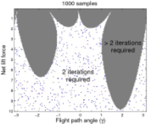
We now describe the applications of the bounds derived in Section 3 to our OAV experiment as described in the introduction. We identify four factors that affect the computational time of the iterative algorithm, and choose 4-dimensional axis-parallel hyper-rectangles as our hypothesis space. The VC dimension of this hypothesis space is 8, as it is known that the VC dimension of axis-parallel hyper-rectangles in Rm is 2m. Thus for δ = .05, ǫ = .05, we need 34,000 samples using Theorem 2.1. But using Theorem 3.8, we need only 1810 samples. With 34,000 samples, if we set δ = .05, ǫ can be as small as 0.0035. The improvement in generalization bound (ǫ) is about 14-fold and in samples complexity (n) is about 18-fold.
The search for the best hyper-rectangle in this experiment is rather simple. For each sampled input, we determine if the iterative algorithm converges. It turns out that in 32,114 instances (roughly 94%), the algorithm converges. Despite this high (empirical) rate of success, in current practice it still loses out to a PID-like controller with fixed deterministic computation time. Next, we randomly choose an axis-parallel 4-dim hyper-rectangle in the input ranges as a hypothesis. If the hyper-rectangle contains a sampled point for which the algorithm does not converge (an unsafe point), then we eliminate that hyper-rectangle (since the guarantees are based on Theorem 3.8 and require zero false positives). Otherwise, we count the number of safe points that lie outside the hyperrectangle (false negatives), and choose the hyper-rectangle that has the fewest number of false negatives. After looking at 10,000 random hyper-rectangles, we are able to come up with one that contains 18,616 safe points and no unsafe points. This hypothesis thus has 32,114 - 18,616 = 13,498 false negatives. Note that the number of false negatives is still quite large. This is because we use hyper-rectangles which constitute a simple hypothesis space that does not approximate the decision surface very well (this SOE is nevertheless a big improvement over the trivial, empty SOE that is the current state of the art). The advantage to this is that the VC dimension is low, and thus only a small number of samples are required to obtain the statistical guarantee, which reads "The found hyper-rectangle has probability of false positive bounded by 0.0035, and we have at least 95% confidence in this statement."
There are a number of alternatives to the above procedure. For example, we can use Corollary 3.6 instead of Theorem 3.8, if the requirement of zero empirical loss is too restrictive. In the OAV example with 34,000 samples, this leads to a hypothesis with 111 false positives but only 3272 false negatives (a reduction of 75%!) while still maintaining 99% confidence that the probability of false positive is less than 0.01. Furthermore, we can replace the criterion "as few false negatives as possible" with other criteria, for example one that prefers hypotheses with large volumes. Finally, if we are willing to make a decision-theoretic tradeoff between false negatives and false positives (e.g. one false positive is as costly as one thousand false negatives), we can set ρ = .001 and apply Corollary 3.5.
5 Summary and RelatedWork
It has been said that the divide between SLT and practice is of Grand Canyon proportions, perhaps because VC bounds are often too loose to be useful in practice. This paper offers a counterargument in the form of an SLT-based approach to verifying complex controllers. We demonstrated this approach on a problem of significant industrial and military interest: Deriving a safe operating envelope for a complex control algorithm. This approach offers control engineers a principled way to increasingly replace low-performance, simple control algorithms with high-performance, complex ones while still maintaining a statistically high confidence in safety. A key to making this offer attractive lies in deriving practical VC-style generalization bounds for weighted binary classification (a problem that hitherto has not been given much attention). Our VC analysis, which builds upon standard VC analysis of unweighted binary classification, shows that such bounds are indeed possible. They are significantly better than a general bound by Vapnik. Our analysis precisely pointed to the place where the false negative penalty had an effect, namely the symmetrization argument. We have successfully applied this verification framework to several other control applications, to be reported in an extended version of this paper. We expect these results to have applications outside of the controller verification problem.
From a practical point of view, SLT-based generalization bounds have been used mostly in the model selection problem (see e.g. [Bartlett et al., 2002]). Aside from this, they have also been used in several control systems applications, for example, in deriving randomized algorithms for robust control problems whose exact solution is NP-hard, and in the context of system identification [Vidyasagar, 2003, Chapter 11]. Also, machine learning researchers have long recognized the importance of learning classifiers with general loss function. The work in this area is generally referred to as cost-sensitive learning [Turney, 2000].
The bounds derived in Section 3 consist of the empirical loss and a VC confidence term that is independent of the probability measure µ and the particular sample Sn. They are thus necessarily "loose" since they need to hold for "bad" distributions and "bad" samples Sn. Recent research has focused on data-based measures of hypothesis space complexity such as Rademacher averages [Koltchinskii, 2001; Bartlett et al., 2005]. This direction relies on Talagrand's approach as described in Section 3.2. Although this approach yields VC dimension-based bounds that have worse constants compared to bounds using the classical approach such as (3.6), it can be used to derive bounds based entirely on data (i.e. Sn) without a priori information about the hypothesis space H (such as its VC dimension d). The following result is an example of such data-dependent bounds.
Theorem 5.1. [Bartlett et al., 2005, Corollary 6.2] Let l = l(ρ) , ρ = 0, 1. Let the random function ˆ ψn be defined on (0, √1/2) as
Then ˆ ψn is sub-root with fixed point ˆ r∗ , and for any α > 0,
Compared to similar result in Section 3.2, the present one is completely data-dependent: In the definition of ˆ ψn(r), the bound 2r/β2 is on the empirical (as opposed to the expected) loss ln(h), and the empirical Rademacher average EσRn (as opposed to ERn) is used. Thus in theory we can obtain a bound without a priori knowledge of the complexity (such as the VC dimension) of the hypothesis space H or of the underlying probability measure µ. However, in practice, computing or estimating ˆ ψn and its fixed point r∗ is far from easy, although Bartlett et al. [2005, Section 6] had made some initial progress in this direction.
Acknowledgements
This work was supported in part by the U.S. Defense Advanced Research Projects Agency (DARPA) and the U.S. Air Force Research Laboratory under Contract No. F33615-01C-1848. We thank Michael Elgersma for help with the OAV experiment, and XuanLong Nguyen for many useful comments.
@inproceedings{ijcai2005p192,
  title     = {Generalization Bounds for Weighted Binary Classification with Applications to Statistical Verification},
  author    = {Ha, Vu and Samad, Tariq},
  booktitle = {Proceedings of the Nineteenth International Joint Conference on
               Artificial Intelligence, {IJCAI-05}},
  publisher = {International Joint Conferences on Artificial Intelligence},
  editor    = {Leslie Pack Kaelbling and Alessandro Saffiotti},
  pages     = {722--726},
  year      = {2005},
  url       = {https://ijcai.org/proceedings/2005/192},
}
TY - CPAPER TI - Generalization Bounds for Weighted Binary Classification with Applications to Statistical Verification AU - Ha, Vu AU - Samad, Tariq T2 - Proceedings of the Nineteenth International Joint Conference on Artificial Intelligence, IJCAI-05 PB - International Joint Conferences on Artificial Intelligence PY - 2005 SP - 722 EP - 726 UR - https://ijcai.org/proceedings/2005/192 ER -Copied
Machine-readable versions of this paper, for tools and AI agents:





