Inferring Image Templates from Classification Decisions

1 Introduction

Consider a psychophysical experiment in which subjects classify a set of images into two classes. The image classes are designed such that correct responses require that the subjects detect the presence of certain features in certain regions of the image. Given the images, and the subjects' classification decisions, is it possible to infer the feature templates the subjects have developed and employed?

This represents an inverse problem in perception, in which the goal is to invert a "direct" model for the subject's responses with the goal of deriving the perceptual features used by the subject. The idea of employing inverse problem techniques is certainly not new in vision research, although it has been initially applied to low-level vision phenomena [Bertero et al., 1988]. The psychological literature on the subject of inverting perceptual similarity data is dominated by research on multidimensional scaling methods (MDS). Metrical MDS [Shepard, 1980] is probably the oldest inversion method allowing the derivation of features from similarities. A neural net-based inversion method for extracting features from judgments of similarity is presented in [Lee, 1998]. More recent work in this direction has addressed the derivation of features involved in higher-level perceptual phenomena [Cutzu and Tarr, 1999; Cutzu, 2000].

The model for the subjects' decisions in the image classification task considered in this work is a generalized nearestneighbor (1-NN) classifier, presented in detail in Section 2. Each of the two image classes is represented by a small set of image templates, or prototypes. Given an input image that must be classified, its degree of match to all templates from all classes is estimated, and its class is determined by the class of the best matching template. Our goal is to infer the prototypes of each class from a set of images labeled by human subjects. Therefore, we are seeking to invert the nearest neighbor problem. This particular inverse problem has received considerable attention in the machine learning community. A comprehensive, recent review of the field is given in [Toussaint, 2002]. One large class of algorithms (Hart's algorithm [Hart, 1968] and its numerous subsequent improvements) selects prototypes from among the labeled data points, a restriction that cannot be applied to our problem due to the presence of pixel noise in the test images.

Our algorithm belongs to the so-called prototype generation methods, which creates prototypes at new locations in feature space. The first such algorithm ([Chang, 1974]) repeatedly merged nearest neighboring points from the same class as long as the classification error rate did not increase. [Bezdek et al., 2001] and later [Mollineda et al., 2002] refined [Chang, 1974] by recursively merging clusters based on geometrical criteria.

The nearest neighbor rule has been generalized by the use of an adaptable metric, a technique also employed in this paper, albeit differently. In [Hastie and Tibshirani, 1996] the metric is locally adapted to the training point neighborhood surrounding the query point at the time of classification. In [Friedman, 1994] also a flexible metric is used for distance calculation in a neighborhood around the query point. However the ideas of recursive partitioning are used in determining the neighborhood for the query point. In [Ricci and Avesani, 1999] a reduced set of prototypes is selected from the training examples and a different metric is associated with each of the selected prototypes. This varies from our approach in two ways. Firstly, the authors in [Ricci and Avesani, 1999] select the prototypes essentially in a random manner. Secondly, we select prototypes that in general do not coincide with the training data points;

A work whose spirit is similar to the present paper is [Xing et al., 2003]: the authors discuss the problem of learning a global (that is, valid throughout feature space) elliptical metric for 1-NN classification from classification data. The metric is fitted to the subject data by solving a convex optimization problem.

2 Amodel for prototype-based image classification

Perceptual considerations required the use of a prototypebased image classifier in which the various prototypes (the image templates) "specialize" in various regions of the image, i.e., a template pays more "attention" to some pixels than to others. This was modeled as follows. Let x ∈ Rd be an input image and ck ∈ Rd one of the templates. This prototype is characterized by a positive (semi) definite matrix Qk which modulates the distance (degree of match) between the template and the image:

The elliptical metric matrix Qk specifies the combination of image pixels the template ck "specializes" in. In the special case where Qk is diagonal, the distance above reduces to:

where Qk(i↪ i) ≥ 0. The pixels i for which Qk(i↪ i) = 0 are ignored by the template ck. This distance measure is termed elliptical. Under the elliptic norm, the set of points (each point in pixel space represents an input image) that lie at equal distance to the prototype is no longer a hypersphere, as for the Euclidean metric, but a hyper-ellipsoid of arbitrary shape and orientation. Each template is characterized by a different ellipsoid. Interestingly, by endowing each prototype with its own, elliptical metric, the resulting Voronoi cells are not necessarily convex or even connected.

An equivalent formulation is derived by using similarity (rather than distance) to prototype: a point is assigned to the most similar prototype. We define the similarity to prototype as the probability of the point "belonging" to the prototype and we associate a Gaussian pdf with each prototype. The shape of the Gaussian varies from prototype to prototype, playing the role of the metric matrix Qk. The similarity of point i to prototype k is, therefore: sik = exp [-(xi - ck)T Qk(xi - ck)] ▷ Or, expressed in Gaussian pdf form:

where the covariance Wk = Q-1 k . Therefore, under the 1NN rule, point xi is assigned to the prototype whose Gaussian is the largest at xi.

3 Finding prototypes for elliptical-metric 1-NN classifiers

Each of the N points xi ∈ Rd (the images) is labeled class 1 or class 2. We seek class-1 and class-2 prototypes which correctly label the N points under the 1-NN rule using the elliptical-norm-based similarity measure in Equation (3). Computing a prototype entails determining its location ck as well as its metric matrix Qk.

Our prototype finding algorithm is as follows:

1. Start with two prototypes, derived by applyingGaussian clusters (algorithm explained below) with two centers to the full data set. Go to step 2.
2. At iteration step t there are Kt prototypes. Consider the points assigned to prototype k (k = 1↪ ▷ ▷ ▷ ↪Kt) by Gaussian clusters. There are nk1 class 1 and nk2 class 2 such points, with nk = nk1 + nk2. If nk1 > nk2, then the prototype is labeled 1, otherwise it is labeled 2. The points of the minority class are, therefore, misclassified by this prototype. The "impurity" of the prototype was defined as the misclassification rate: rk =
3. 1 - max [ nk1 nk ↪ nk2 nk ]. If the impurity of prototype k is
4. greater than some user-defined threshold g, rk > g, then prototype k is considered for being split into two prototypes (just like a node in a classification tree is split when too impure). The splitting is performed only if the splitting reduces the impurities in the two resulting clusters. If a node does get split, we obtain a class 1 and a class 2 prototype. These "child" prototypes are placed at the centers of mass of the nk1, respective nk2 points. Due to splitting, at the end of this step there are Kt+1 ≥ Kt prototypes.

If no prototypes are split, go to Step 4, else go to Step 3.

1. Re-apply Gaussian clusters to the data set, ignoring point labels. Gaussian clusters is initialized with the Kt+1 prototypes determined at Step 2. Go to Step 2.
2. The algorithm also returns a global classification error rate which measures the errors caused by using the prototypes for classification. This error rate is defined by the total number of minority class points at all prototypes. The prototypes are labeled according to the majority class at the prototype. Thus, for each prototype a center (ck), a covariance matrix (Wk), and a class label are returned.

Observations: i) The algorithm has as sole adjustable parameter the impurity threshold g. The number of prototypes of either class is determined automatically. ii) The class labels of the points are solely used in splitting decisions, and are irrelevant to the Gaussian k-means algorithm. iii) Note the similarity to classification and regression trees (CART).

The Gaussian clusters algorithm fits K Gaussian clusters to input data set. The Gaussian clusters algorithm is basically like k-means clustering except that each center also has a covariance matrix associated with it. So for every iteration of the Gaussian clusters algorithm when the new centers are being estimated we also estimate the new covariance matrices. This covariance matrix distorts the attraction of each center along the different dimensions.

4 Results: Artificial data

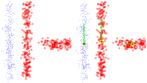
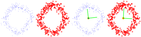
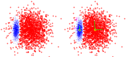
We applied our prototype finding algorithm to several synthetic data sets, illustrated in Figures 1-3. These synthetic data sets were generated in two dimensions (two pixel images), so that the structure of the point clouds are clearly visible.

In experiment 1 (Figure 1) there were 320 points of class 1 (blue) and 380 points of class 2 (red). The class 1 points were arranged in a single vertical band and the class 2 points were shared by 1 vertical and 1 horizontal band. As expected three centers have been assigned to the three distinct point clouds based on the desired purity tolerance.

In experiment 2 (Figure 2) there were 340 points of class 1 (blue) and 340 points of class 2 (red). The points were arranged into two non-overlapping, non-concentric circles. As seen in the figure two prototypes were assigned, one to each circle. Note that the prototype centers are at locations where there were no training examples.

In experiment 3 (Figure 3), there were 1849 points of class 1 (blue) and 1849 points of class 2 (red). Both the classes were drawn from a gaussian distribution, with different means and standard deviations. Notice the overlap of the two point clouds. In the results obtained from the algorithm, we can see that the points assigned to the class 2 prototype surround the class 1 cluster: this non-convexity is an effect of the elliptical norm in determining nearest-neighbors.

5 Results: Psychophysical experiment data

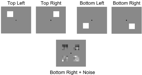
The prototype finding algorithm was applied to simulated data and also to human image classification data collected in a psychophysical experiment in which the subjects had to discriminate between two classes of visual patterns. The visual pattern discrimination task is illustrated in Figure 4. In this task, the observer is shown a single white square corrupted by additive Gaussian pixel noise at one of four possible locations. The location of the square is randomly chosen on each trial. Two of the possible locations are above the fixation point and two are below the fixation point, with each location being equidistant from the central fixation point. Noise is added to each pixel in each of the four locations, with each location divided into a 4×4 grid of pixels. No noise is added to the regions in between the four square locations, and the fixation point remains on the screen throughout the experiment. The observers task is to indicate whether the white square signal appeared above or below fixation. The contrast of the white square is manipulated across trials according to a 2-down 1-up adaptive staircase procedure to place it at a level where performance is at approximately 71% correct. Accuracy feedback is given in the format of a high or low beep.

Before collecting human subject data two simulations were performed using the above experimental setup. The two models simulated were the "exemplar" model and the "prototype" model. In an "exemplar" model the observers are assumed to use multiple noisy "templates" to form a representation for each category. Each of these templates are compared to the input to reach a classification decision. The templates used in the "exemplar" model simulation were the ideal templates (the four signals shown in Figure 4). In a "prototype" model observers are assumed to use a single summary representation for each category. Thus the templates used in the prototype model simulation were combined versions of the two signals within each category. This resulted in a 'top' prototype template composed of the two top squares and a 'bottom' prototype template composed of the two bottom squares. For each of these two models a simulation with 16000 trials was performed.

Four human subjects were tested. For each subject, 4000 experimental trials were conducted. The staircase procedure was used to keep the performance rate for each subject pegged at around 71% correct.

Since each white square was 4×4 pixels, the classification images viewed by the subjects were 8 × 8 pixels (the center of the display was a constant gray-level). Therefore, the algorithm learned prototypes in 64-dimensional space. The simplifying assumption was made that there were no perceptual interactions between the pixels, and therefore the covariance matrices associated with the prototypes were restricted to being diagonal. A diagonal covariance matrix has one entry per pixel, and can be interpreted as an image-sized mask that indicates which pixels the corresponding prototype pays attention (responds) to.

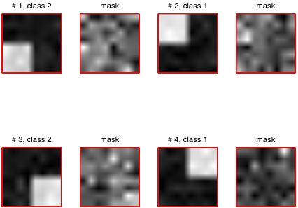
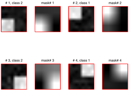
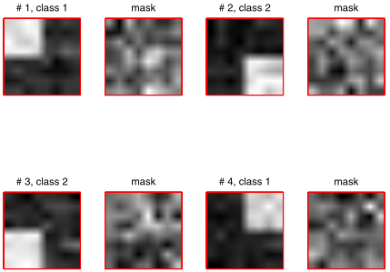
The algorithm yielded the expected templates when applied to the simulation data. Figure 5 1 shows the templates obtained on running the algorithm on the "exemplar" model simulation. As expected the centers represent the four different stimuli. The masks shown alongside each center show the relative importance of each pixel for that template. The masks are actually the inverses of the diagonal values of the diagonal covariance matrices. A whiter pixel in the mask indicates that the template is more sensitive to that particular pixel. The masks are quite noisy but one can see that the pixels of the image that include the stimuli are considered more important by the mask. To show the relative importance of each of the four quadrants we also displayed the masks averaged over each of the four quadrants (Figure 6). In this figure the higher importance of the quadrant containing the stimulus is clearly visible.

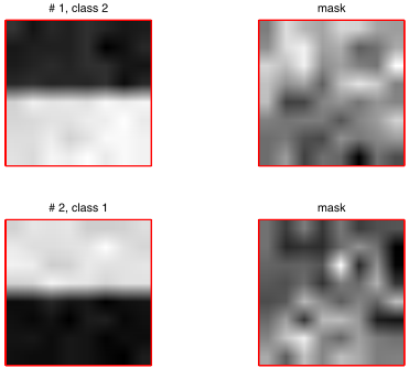
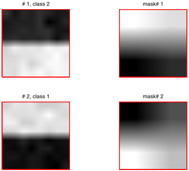
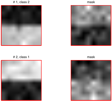
Figure 7 shows the templates obtained on running the algorithm on the "prototype" model simulation. As expected the two centers represent the combination of the stimuli that form each class. The masks shown alongside each center show the relative importance of each pixel for that template. The masks are again quite noisy but one can see that the pixels of the image that do not include the stimuli are considered more important by the mask. To show the relative importance of each of the four quadrants we also displayed the masks averaged over each of the four quadrants (Figure 8). In this figure the higher importance of the quadrants not containing the stimulus is clearly visible.

1 The results (Figures 5 - 12) are displayed in a more concise format than the format (example Figure 4) used during experiments. In particular, the "fixation point" is not shown and the four, 4 × 4 pixel squares are shown adjacent to each other in the results.

The difference in the behavior of the mask across the "exemplar" and "prototype" simulations is interesting. In the case of the "prototype" simulation it seems that the classification into top (class 1) is made by the presence of darker pixels in both the bottom quadrants and vice versa.

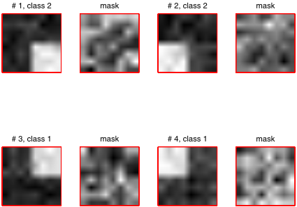
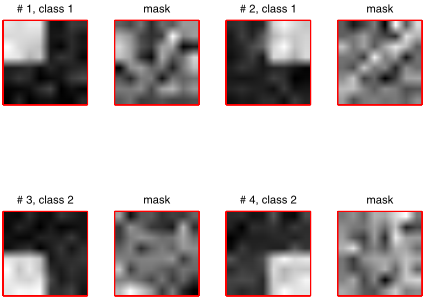
The algorithm yielded interesting results on the human subjects. Three subjects (subjects 1,3 and 4) appeared to have used four centers, one for each corner square, and thus two per class, as can be seen in Figures 9, 11, 12. The masks obtained for the subject data show that the pixels considered most important do not seem to follow any particular pattern. Also the difference in importance across pixels is very small. This seems to lead to the conclusion that the human subjects based their decision on the entire image rather than on a particular quadrant.

Interestingly, subject two appears to have used two centers, one per class (Figure 10). The two centers correspond to the two top and bottom corners taken together. Note that in no actual stimulus both corner squares are "on" simultaneously. This would correspond, in the language of the psychology of categorization, to a so-called "prototype model", while the other three subjects operated using an "exemplar model". The masks in this case are more distinct and like in the "prototype" simulation show a stronger response for the pixels in which the stimulus is absent. This can intuitively be explained by noting that for example in class 'top' no input image actually contains a stimulus in both the 'top left' and the 'top right' quadrant. However for class 'top' both the bottom quadrants can be expected to have a lower contrast value, because the stimulus is absent in the lower two quadrants. A similar intuition can be applied to the 'bottom' class.

6 Discussion

We introduced a prototype generating method for nearestneighbor classification. Each prototype is endowed with its own elliptical metric, and our method is therefore related to adaptive metric methods such as [Hastie and Tibshirani,

1996] and especially [Xing et al., 2003]. The prototypes are not a subset of the data points, and therefore our method belongs in the prototype generation category. However, as opposed to Chang's method and its later refinements ([Bezdek et al., 2001], [Mollineda et al., 2002]) we find new prototypes by recursively splitting clusters, rather than by aggregating them.

The main contribution of this paper lies in the application of the prototype learning algorithm to understanding human image classification. If an image classification experiment is designed such that correct classification decisions require the detection of one of several class-specific features in certain regions of the image, then nearest-neighbor is an appropriate classification model. In the experiment described in this paper, class 1 was defined by the presence of feature A (Top Left) or feature B (Top Right) and class 2 by the presence of feature C (Bottom Left) or feature D (Bottom Right). Any image contains only one of the four features, and, moreover, each feature occupies a specific image region. The algorithm correctly identified the regions of the image each prototype "specializes" in.

In this situation, there are two equally effective decision strategies available to a nearest-neighbor classifier: 1. store two prototypes per class, one for each of the features A, B, C, D; or, 2. store one prototype per class, one for the composite feature (A or B) and one for the composite feature (C or D). The first strategy corresponds, in the terminology of the psychology of categorization, to categorization by exemplar, and the second, to categorization by prototype. Most interestingly, our algorithm revealed that one of the subjects employed the second strategy, and the other three the first. It is important to note that a conventional analysis of error rates would not be able to distinguish between the two strategies.