
Affine Algebraic Decision Diagrams (AADDs) and their Application to Structured Probabilistic Inference
Proceedings of the Nineteenth International Joint Conference on Artificial Intelligence. Pages 1384-1389.
© 2005 International Joint Conferences on Artificial Intelligence
Abstract
We propose an affine extension to ADDs (AADD) capable of compactly representing context-specific, additive, and multiplicative structure. We show that the AADD has worstcase time and space performance within a multiplicative constant of that of ADDs, but that it can be linear in the number of variables in cases where ADDs are exponential in the number of variables. We provide an empirical comparison of tabular, ADD, and AADD representations used in standard Bayes net and MDP inference algorithms and conclude that the AADD performs at least as well as the other two representations, and often yields an exponential performance improvement over both when additive or multiplicative structure can be exploited. These results suggest that the AADD is likely to yield exponential time and space improvements for a variety of probabilistic inference algorithms that currently use tables or ADDs.
- R.I. Bahar, E.A. Frohm, C.M. Gaona, G.D. Hachtel, E. Macii, A. Pardo, F. Somenzi: Algebraic Decision Diagrams and Their Applications. ICCAD. (1993)
- Boutilier, C., Friedman, N., Goldszmidt, M., Koller, D.: Context-specific independence in Bayesian net- works. UAI. (1996)
- Drechsler, R., Sieling, D.: BDDs in theory and practice. Software Tools for Technology Transfer. (2001)
- Bryant, R.E.: Graph-based algorithms for Boolean func- tion manipulation. IEEE Trans. on Computers. (1986)
- Rudell, R.: Dynamic variable ordering for ordered bi- nary decision diagrams. ICCAD. (1993)
- Zhang, N.L., Poole, D.: A simple approach to bayesian network computations. CCAI. (1994)
- Takikawa, M., D'Ambrosio, B.: Multiplicative factor- ization of noisy-max. UAI. (1999)
- Bellman, R.E.: Dynamic Programming. Princeton Uni- versity Press, Princeton, NJ (1957)
- Hoey, J., St-Aubin, R., Hu, A., Boutilier, C.: SPUDD: Stochastic planning using decision diagrams. UAI. (1999)
- Guestrin, C., Koller, D., Parr, R.: Max-norm projec- tions for factored MDPs. IJCAI. (2001) IJCAI
References were extracted automatically from the PDF and may contain errors.
Full text extracted automatically from the PDF; figures, tables and equations may differ. The PDF is the version of record.
1 Introduction
Algebraic decision diagrams (ADDs) [1] provide an efficient means for representing and performing arithmetic operations on functions from a factored boolean domain to a real-valued range (i.e., Bn →R). They rely on two main principles to do this:
- ADDs represent a function Bn → R as a directed acyclic graph - essentially a decision tree with reconvergent branches and real-valued terminal nodes.
- ADDs enforce a strict variable ordering on the decisions from the root to the terminal node, enabling a minimal, canonical diagram to be produced for a given function. Thus, two identical functions will always have identical ADD representations under the same variable ordering.
As shown in Figure 1, ADDs often provide an efficient representation of functions with context-specific independence [2], such as functions whose structure is conjunctive (1a) or disjunctive (1b) in nature. Thus,
David McAllester
TTI at Chicago 1427 East 60th Street Chicago, IL 60637, USA
mcallester@tti-c.org
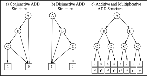
ADDs can offer exponential space savings over a fully enumerated tabular representation. However, the compactness of ADDs does not extend to the case of additive or multiplicative independence, as demonstrated by the exponentially large representations when this structure is present (1c). Unfortunately such structure often occurs in probabilistic and decision-theoretic reasoning domains, potentially leading to exponential running times and space requirements for inference in these domains.
2 Affine Algebraic Decision Diagrams
To address the limitations of ADDs, we introduce an affine extension to the ADD (AADD) that is capable of canonically and compactly representing context-specific, additive, and multiplicative structure in functions from Bn →R. We define AADDs with the following BNF:
Here, ch and cl are real (or floating-point) constants in the closed interval [0, 1], bh and bl are real constants in the half-open interval (0, 1], F var is a boolean variable associated with F, and Fl and Fh are non-terminals of type F. We also impose the following constraints:
- The variable F var does not appear in Fh or Fl.
- min(ch, cl) = 0
- max(ch + bh, cl + bl) = 1
- If Fh = 0 then bh = 0 and ch > 0. Similarly for Fl.
- In the grammar for G, we require that if F = 0 then b = 0, otherwise b > 0.
Expressions in the grammar for F will be called normalized AADDs and expressions in the grammar for G will be called generalized AADDs.1
Let V al(F, ρ) be the value of AADD F under variable value assignment ρ. This can be defined recursively by the following equation:
We say that F satisfies a given variable ordering if F = 0 or F is of the form if(F var , ch + bhFh, cl + blFl) where F var does not occur in Fh or Fl and F var is the earliest variable under the given ordering occuring in F. We say that a generalized AADD of form c+bF satisfies the order if F satisfies the order.
Lemma 2.1. For any normalized AADD F we have that V al(F, ρ) is in the interval [0, 1], minρ V al(F, ρ) = 0, and if F ̸= 0 then maxρ V al(F, ρ) = 1.
Lemma 2.2. Fix a variable ordering. For any nonconstant function g mapping Bn -→ R, there exists a unique generalized AADD G satisfying the given variable ordering such that for all ρ ∈ Bn we have g(ρ) = V al(G, ρ).
Both lemmas can be proved by straightforward induction on n. The second lemma shows that under a given variable ordering, generalized AADDs are canonical, i.e., two identical functions will always have identical AADD representations.
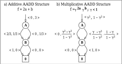
As an example of two AADDs with compact additive and multiplicative structure, Figure 2 shows portions of the exponentially sized ADDs from Figure 1c represented by generalized AADDs of linear size.
1Since normalized AADDs in grammar F are restricted to the range [0, 1], we need the top-level positive affine transform of generalized AADDs in grammar G to allow for the representation of functions with arbitrary range.
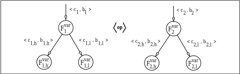
We let op denote a binary operator on AADDs with possible operations being addition, substraction, multiplication, division, min, and max denoted respectively as ⊕, ⊖, ⊗, ⊘, min(·, ·), and max(·, ·).
3 Related Work
There has been much related work in the formal verification literature that has attempted to tackle additive and multiplicative structure in representation of functions from Bn →Bm. These include *BMDs, K*BMDs, EVBDDs, FEVBDDs, HDDs, and *PHDDs [3]. While space limitations prevent us from discussing all of the differences between AADDs and these data structures, we note two major differences: 1) These data structures have different canonical forms relying on GCD factorization and do not satisfy the invariant property of AADDs that internal nodes have range [0, 1]. 2) The fact that these data structures have integer terminals (Bm) requires a rational or direct floating-point representation of values in R. In our experience, this renders them unusable for probabilistic inference due to considerable numerical precision error and computational difficulties.
4 Algorithms
We now define AADD algorithms that are analogs of those given by Bryant [4]2 except that they are extended to propagate the affine transform of the edge weights on recursion and to compute the normalization of the resulting node on return.
All algorithms rely on the helper function GetGNode given in Algorithm 1 that takes an unnormalized AADD node of the form if(v, ch+bhFh, cl+blFl) and returns the cached, generalized AADD node of the form 〈cr+brFr〉.3
4.1 Reduce
The Reduce algorithm given in Algorithm 2 takes an arbitrary ordered AADD, normalizes and caches the internal nodes, and returns the corresponding generalized AADD. One nice property of the Reduce algorithm is that one does not need to prespecify the structure that
2Bryant gives algorithms for binary decision diagrams (BDDs), but they are essentially identical to those for ADDs.
3 In the algorithms we use the representation 〈c, b, F〉, while in the text we often use the equivalent notation 〈c+bF〉 to make the node semantics more clear.
Algorithm 1: GetGNode(v, 〈ch, bh, Fh〉, 〈cl, bl, Fl〉) -→ 〈cr, br, Fr〉input : v, 〈ch, bh, Fh〉, 〈cl, bl, Fl〉 : Var, offset, mult, and node id for high/low branches output : 〈cr, br, Fr〉 : Return values for offset, multiplier, and canonical node id begin // If branches redundant, return child if (cl = ch ∧ bl = bh ∧ Fl = Fh) then return 〈cl, bl, Fl〉; // Non-redundant so compute canonical form rmin :=min(cl, ch); rmax :=max(cl + bl, ch + bh); rrange := rmax - rmin; cl := (cl - rmin)/rrange; ch := (ch - rmin)/rrange; bl := bl/rrange; bh := bh/rrange; if (〈v, 〈ch, bh, Fh〉, 〈cl, bl, Fl〉〉 → id is not in node cache) then id := currently unallocated id; insert 〈v, 〈ch, bh, Fh〉, 〈cl, bl, Fl〉〉 → id in cache; // Return the cached, canonical node return 〈rmin, rrange, id〉 ; endthe AADD should exploit. If the represented function contains context-specific, additive, or multiplicative independence, the Reduce algorithm will compactly represent this structure uniquely and automatically w.r.t. the variable ordering as guaranteed by previous lemmas.
4.2 Apply
The Apply routine given in Algorithm 3 takes two generalized AADD operands and an operation as given in Figure 3 and produces the resulting generalized AADD. The control flow of the algorithm is straightforward: We first check whether we can compute the result immediately, otherwise we normalize the operands to a canonical form and check if we can reuse the result of a previously cached computation. If we can do neither of these, we then choose a variable to branch on and recursively call the Apply routine for each instantiation of the variable. We cover these steps in-depth in the following sections.
Terminal computation
The function ComputeResult given in the top half of Table 1, determines if the result of a computation can be immediately computed without recursion. The first entry in this table is required for proper termination of the algorithm as it computes the result of an operation applied to two terminal 0 nodes. However, the other entries denote a number of pruning optimizations that immediately return a node without recursion. For example, given the operation 〈3+4F1〉⊕〈5+6F1〉, we can immediately return the result 〈8+10F1〉.
Recursive computation
If a call to Apply is unable to immediately compute a result or reuse a previously cached computation, we must recursively compute the result. For this we have two
Algorithm 2: Reduce(〈c, b, F 〉) -→ 〈cr, br, Fr〉input : 〈c, b, F〉 : Offset, multiplier, and node id output : 〈cr, br, Fr〉 : Return values for offset, multiplier, and node id begin // Check for terminal node if (F = 0) then return 〈c, 0, 0〉; // Check reduce cache if ( F → 〈cr, br, Fr〉 is not in reduce cache) then // Not in cache, so recurse 〈ch, bh, Fh〉 := Reduce(ch, bh, Fh); 〈cl, bl, Fl〉 := Reduce(cl, bl, Fl); // Retrieve canonical form 〈cr, br, Fr〉 := GetGNode(F var , 〈ch, bh, Fh〉, 〈cl, bl, Fl〉); // Put in cache insert F → 〈cr, br, Fr〉 in reduce cache; // Return canonical reduced node return 〈c + b · cr, b · br, Fr〉; endcases (the third case where both operands are 0 terminal nodes having been taken care of in the previous section):
F1 or F2 is a 0 terminal node, or F var 1 ̸= F var 2 : We assume the operation is commutative and reorder the operands so that F1 is the 0 node or the operand whose variable comes later in the variable ordering.4 Then we propagate the affine transform to each of F2's branches and compute the operation applied separately to F1 and each of F2's high and low branches. We then build an if statement conditional on F var 2 and normalize it to obtain the generalized AADD node 〈cr, br, Fr〉 for the result:
F1 and F2 are non-terminal nodes and F var 1 = F var 2 : Since the variables for each operand match, we know the result 〈cr, br, Fr〉 is simply a generalized if statement branching on F var 1 (= F var 2 ) with the true case being the operator applied to the high branches of F1 and F2 and likewise for the false case and the low branches:
4We note that the first case prohibits the use of the noncommutative ⊖ and ⊘ operations. However, a simple solution would be to recursively descend on either F1 or F2 rather than assuming commutativity and swapping operands to ensure descent on F2. To accommodate general non-commutative operations, we have used this alternate approach in our specification of the Apply routine given in Algorithm 3.
Canonical caching
If the AADD Apply algorithm were to compute and cache the results of applying an operation directly to the operands, the algorithm would provably have the same time complexity as the ADD Apply algorithm. Yet, if we were to compute 〈0+1F1〉⊕〈0+2F2〉 and cache the result 〈cr + brFr〉, we could compute 〈5 + 2F1〉 ⊕ 〈4 + 4F2〉 = 〈(2cr + 9) + 2brFr〉 without recursion.
This suggests a canonical caching scheme that normalizes all cache entries to increase the chance of a cache hit. The actual result can then be easily computed from the cached result by reversing the normalization. This ensures optimal reuse of the Apply operations cache and can lead to an exponential reduction in running time over the non-canonical caching version.
We introduce two additional functions to perform this caching: GetNormCacheKey to compute the canonical cache key, and ModifyResult to reverse the normalization in order to compute the actual result. These algorithms are summarized in the bottom half of Table 1.
4.3 Other Operations
While space limitations prevent us from covering all of the operations that can be performed (efficiently) on AADDs, we briefly summarize some of them here:
min and max computation: The min and max of a generalized AADD node 〈c + bF〉 are respectively c and c + b due to [0, 1] normalization of F.
Restriction: The restriction of a variable xi in a function to either true or false (i.e. F|xi=T/F ) can be computed by returning the proper branch of nodes containing that test variable during the Reduce operation.
Sum out/marginalization: A variable xi can be summed (or marginalized) out of a function F simply by computing the sum of the restricted functions (i.e. F |xi=T ⊕ F |xi=F ).
Variable reordering: A generalization of Rudell's ADD variable reordering algorithm [5] that recomputes edge weights of reordered nodes can be applied to AADDs without loss of efficiency.
Negation/reciprocation: While it may seem that negation of a generalized AADD node 〈c + bF〉 would be as simple as 〈-c + -bF〉, we note that this violates our normalization scheme which requires b > 0. Consequently, negation must be performed explicitly as 0⊖ 〈c + bF〉. Likewise, reciprocation (i.e., 1 〈c+bF 〉 ) must be performed explicitly as 1 ⊘ 〈c + bF〉.
4.4 Cache Implementation
If one were to use a naive cache implementation that relied on exact floating-point values for hashing and equality testing, one would find that many nodes which should be the same under exact computation often turn out to have offsets or multipliers differing by ±1e-15 due to numerical precision error. This can result in an exponential explosion of nodes if not controlled. Consequently, it is better to use a hashing scheme that considers equality within some range of numerical precision error ϵ. While
Algorithm 3: Apply(〈c1, b1, F1〉, 〈c2, b2, F2〉, op) -→ 〈cr, br, Fr〉input : 〈c1, b1, F1〉, 〈c2, b2, F2〉, op : Nodes and op output : 〈cr, br, Fr〉 : Generalized node to return begin // Check if result can be immediately computed if (ComputeResult(〈c1, b1, F1〉, 〈c2, b2, F2〉, op) → 〈cr, br, Fr〉 is not null ) then return 〈cr, br, Fr〉; // Get normalized key and check apply cache 〈〈c′1, b′1〉, 〈c′2, b′2〉〉 := GetNormCacheKey(〈c1, b1, F1〉, 〈c2, b2, F2〉, op); if ( 〈〈c′1, b′1, F1〉, 〈c′2, b′2, F2〉, op〉 → 〈cr, br, Fr〉 is not in apply cache) then // Not terminal, so recurse if (F1 is a non-terminal node) then if (F2 is a non-terminal node) then if (F var 1 comes before F var 2 ) then var := F var 1 ; elsevar := F var 2 ; elsevar := F var 1 ; elsevar := F var 2 ; // Propagate affine transform to branches if (F1 is non-terminal ∧ var = F var 1 ) then F v1 l := F1,l; F v1 h := F1,h; cv1 l := c′1 + b′1 · c1,l; cv1 h := c′1 + b′1 · c1,h; bv1 l := b′1 · b1,l; bv1 h := b′1 · b1,h; elseF v1 l/h := F1; cv1 l/h := c′1; bv1 l/h := b′1; if (F2 is non-terminal ∧ var = F var 2 ) then F v2 l := F2,l; F v2 h := F2,h; cv2 l := c′2 + b′2 · c2,l; cv2 h := c′2 + b′2 · c2,h; bv2 l := b′2 · b2,l; bv2 h := b′1 · b2,h; elseF v2 l/h := F2; cv2 l/h := c′2; bv2 l/h := b′2; // Recurse and get cached result 〈cl, bl, Fl〉 :=Apply(〈cv1 l , bv1 l , F v1 l 〉, 〈cv2 l , bv2 l , F v2 l 〉, op); 〈ch, bh, Fh〉 :=Apply(〈cv1 h , bv1 h , F v1 h 〉, 〈cv2 h , bv2 h , F v2 h 〉, op); 〈cr, br, Fr〉 := GetGNode(var, 〈ch, bh, Fh〉, 〈cl, bl, Fl〉); // Put result in apply cache and return insert 〈c′1, b′1, F1, c′2, b′2, F2, op〉 → 〈cr, br, Fr〉 into apply cache; return ModifyResult(〈cr, br, Fr〉); endit is difficult to guarantee such an exact property for an efficient hashing scheme, we next outline an approximate approach that we have found to work both efficiently and nearly optimally in practice.
The node cache used in GetGNode and the operation result cache used in Apply both use cache keys containing four floating-point values (i.e., the offsets and multipliers
| ComputeResult(〈c1, b1, F1〉, 〈c2, b2, F2〉, op) -→ 〈cr, br, Fr〉 | |
|---|---|
| Operation and Conditions | Return Value |
| 〈c1 + b1F1〉 〈op〉 〈c2 + b2F2〉; F1 = F2 = 0 | 〈(c1 〈op〉 c2) + 0 · 0〉 |
| max(〈c1 + b1F1〉, 〈c2 + b2F2〉); c1 + b1 ≤ c2 | 〈c2 + b2F2〉 |
| max(〈c1 + b1F1〉, 〈c2 + b2F2〉); c2 + b2 ≤ c1 | 〈c1 + b1F1〉 |
| 〈c1 + b1F1〉 ⊕ 〈c2 + b2F2〉; F1 = F2 | 〈(c1 + c2) + (b1 + b2)F1〉 |
| max(〈c1 + b1F1〉, 〈c2 + b2F1〉); F1 = F2, (c1 ≥ c2 ∧ b1 ≥ b2) ∨ (c2 ≥ c1 ∧ b2 ≥ b1) | c1 ≥ c2 ∧ b1 ≥ b2 : 〈c1 + b1F1〉 c2 ≥ c1 ∧ b2 ≥ b1 : 〈c2 + b2F1〉 |
| Note: for all max operations above, return opposite for min | |
| 〈c1 + b1F1〉 〈op〉 〈c2 + b2F2〉; F2 = 0, op ∈ {⊕,⊖} | 〈(c1 〈op〉 c2) + b1F1〉 |
| 〈c1 + b1F1〉 〈op〉 〈c2 + b2F2〉; F2 = 0, c2 ≥ 0, op ∈ {⊗,⊘} | 〈(c1 〈op〉 c2) + (b1 〈op〉 c2)F1〉 |
| Note: above two operations can be modified to handle F1 = 0 when op ∈ {⊕,⊗} | |
| other | null |
| GetNormCacheKey(〈c1, b1, F1〉, 〈c2, b2, F2〉, op) -→ 〈〈c′1, b′1〉〈c′2, b′2〉〉 and ModifyResult(〈cr, br, Fr〉) -→ 〈c′r, b′r, F ′r〉 | ||
|---|---|---|
| Operation and Conditions | Normalized Cache Key and Computation | Result Modification |
| 〈c1 + b1F1〉 ⊕ 〈c2 + b2F2〉; F1 ̸= 0 | 〈cr + brFr〉 = 〈0+1F1〉 ⊕ 〈0+ (b2/b1)F2〉 | 〈(c1 + c2 + b1cr) + b1brFr〉 |
| 〈c1 +b1F1〉 ⊖ 〈c2 +b2F2〉; F1 ̸= 0 | 〈cr + brFr〉 = 〈0+1F1〉 ⊖ 〈0+ (b2/b1)F2〉 | 〈(c1 - c2 + b1cr) + b1brFr〉 |
| 〈c1 + b1F1〉 ⊗ 〈c2 + b2F2〉; F1 ̸= 0 | 〈cr + brFr〉 = 〈(c1/b1) +F1〉 ⊗ 〈(c2/b2) +F2〉 | 〈b1b2cr + b1b2brFr〉 |
| 〈c1 + b1F1〉 ⊘ 〈c2 + b2F2〉; F1 ̸= 0 | 〈cr + brFr〉 = 〈(c1/b1) +F1〉 ⊘ 〈(c2/b2) +F2〉 | 〈(b1/b2)cr + (b1/b2)brFr〉 |
| max(〈c1 + b1F1〉, 〈c2 + b2F2〉); F1 ̸= 0, Note: same for min | 〈cr + brFr〉 =max(〈0+1F1〉, 〈(c2 - c1)/b1 + (b2/b1)F2〉) | 〈(c1 + b1cr) + b1brFr〉 |
| any 〈op〉 not matching above: + + | 〈cr + brFr〉 = 〈c1 + b1F1〉 〈op〉 〈c2 + b2F2〉 | 〈cr + brFr〉 |
〈c1 + b1F1〉 〈op〉 〈c2 + b2F2〉
Table 1: Input and output summaries of the ComputeResult, GetNormCacheKey, and ModifyResult routines.
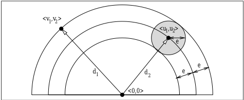
for two AADD nodes). If we consider this 4-tuple of floating-point values to be a point in Euclidean space, then we can measure the error between two 4-tuples 〈u1, u2, u3, u4〉 and 〈v1, v2, v3, v4〉 as the L2 (Euclidean) distance between these points. As a consequence of the triangle inequality for four dimensions, we know that √(u1 - v1)2 + (u2 - v2)2 + (u3 - v3)2 + (u4 - v4)2 ≤ ϵ ⇒|√u1 2 + u2 2 + u3 2 + u4 2 -√v1 2 + v2 2 + v3 2 + v4 2 | ≤ ϵ. This is shown graphically for two dimensions in Figure 4.
Based on this inequality, we can use the following approximate hashing scheme for 〈v1, v2, v3, v4〉: Compute the L2 distance between 〈v1, v2, v3, v4〉 and the origin; For hashing, extract only the bits from the floating-point base representing a fractional portion greater than ϵ and use this as the integer representation of the hash key (we are effectively discretizing the distances into buckets of width ϵ); For equality, test that the true L2 metric between 〈u1, u2, u3, u4〉 and 〈v1, v2, v3, v4〉 is less than ϵ.
While this hashing scheme does not guarantee that all 4-tuples having distance from the origin 〈0, 0, 0, 0〉 within ϵ hash to the same bucket (some 4-tuples within ϵ could fall over bucket boundaries), we found that with bucket width ϵ = 1e-9 and numerical precision error generally less than 1e-13, there was only a small probability of two nodes equal within numerical precision straddling a bucket boundary. For the empirical results described in Section 6, this hashing scheme was sufficient to prevent any uncontrollable cases of numerical precision error.
5 Theoretical Results
Here we present two fundamental results for AADDs:
Theorem 5.1. The time and space performance of Reduce and Apply for AADDs is within a multiplicative constant of that of ADDs in the worst case.
Proof Sketch. Under the same variable ordering, an ADD is equivalent to a non-canonical AADD with fixed edge weights c = 0, b = 1. Thus the ADD Reduce and Apply algorithms can be seen as analogs of the AADD algorithms without the additional constant-time probability tables (CPTs) Pj and corresponding operations replaced with those for tables, ADDs, and AADDs:
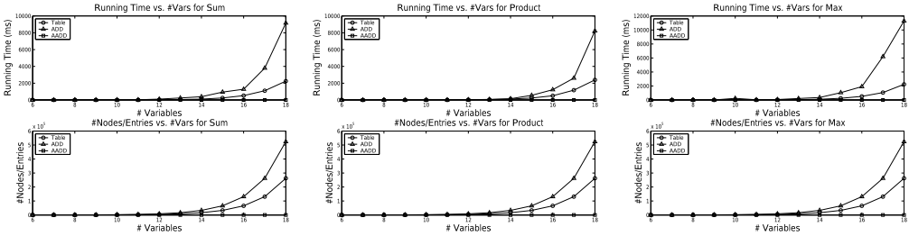
Table 2 shows the total number of table entries/nodes required to represent the original network and the total running time of 100 random queries (each consisting of one query variable and one evidence variable) for a number of publicly available BNs (http://www.cs.huji.ac.il/labs/compbio/Repository) and two noisy-or and noisy-max CPTs with 15 parent nodes.
Note that the intermediate probability tables were often too large for the tables or ADDs, but not the AADDs, indicating that the AADD was able to exploit additive or multiplicative structure in these cases. Also, the AADD yields an exponential to linear reduction on the Noisy-Or-15 problem and a considerable computational speedup on the Noisy-Max-15 problem by exploiting the additive and multiplicative structure inherent in these special CPTs [7].
6.3 Markov Decision Processes
For MDPs, we simply evaluate the value iteration algorithm [8] using a tabular representation and its extension for decision diagrams [9] to factored MDPs from the SysAdmin domain [10].5 Here we simply substitute tables, ADDs, and AADDs for the reward function R, value function V , and transition model dynamics Pi in the following factored MDP value iteration update:
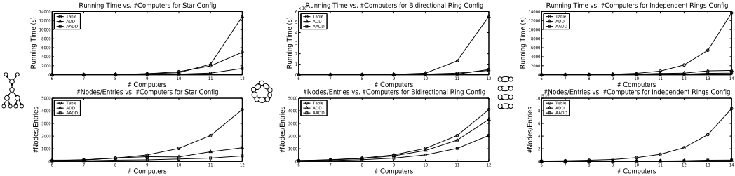
Figure 6 shows the relative performance of value iteration until convergence within 0.01 of the optimal value
5 In these domains, there is a network of computers whose operational status (i.e., running or crashed) at each time step is a stochastic function of the previous status of computers with incoming connections. At each time step the task of the system administrator is to choose the computer to reboot in order to maximize the sum of operational computers over a discounted reward horizon.
and constant-space overhead of normalization. Since normalization can only increase the number of Reduce and Apply cache hits and reduce the number of cached nodes, it is clear that an AADD must generate equal or fewer Reduce and Apply calls and have equal or fewer cached nodes than the corresponding ADD. This allows us to conclude that in the worst case where the AADD generates as many Reduce and Apply calls and cache hits as the ADD, the AADD is still within a multiplicative constant of the time and space required by the ADD.
Theorem 5.2. There exist functions F1 and F2 and an operator op such that the running time and space performance of Apply(F1, F2, op) for AADDs can be linear in the number of variables when the corresponding ADD operations are exponential in the number of variables.
Proof Sketch. Two functions and Apply operation examples where this holds true are ∑ni=1 2ixi⊕ ∑ni=1 2ixi and ∏ni=1 γ 2i xi ⊗ ∏ni=1 γ 2i xi . (Examples of these operands as ADDs and AADDs were given in Figures 1c and 2.) Because these computations result in a number of terminal values exponential in n, the ADD operations must require time and space exponential in n. On the other hand, it is known that the operands can be represented in linear-sized AADDs. Due to this structure, the Apply algorithm will begin by recursing on the high branch of both operands to depth n. Then, at each step as it returns and recurses down the low branch, the respective additive and multiplicative differences will be normalized out due to the canonical caching scheme, thus yielding cache hits for all low branches. This results in n cached nodes and 2n Apply calls for the AADD operations.
6 Empirical Results
6.1 Basic Operations
Figure 5 demonstrates the relative time and space performance of tables, ADDs, and AADDs on a number of basic operations. These verify the exponential to linear space and time reductions proved in Theorem 5.2.
6.2 Bayes Nets
For Bayes nets (BNs), we simply evaluate the variable elimination algorithm [6] (under a fixed, greedy treewidth minimizing variable ordering) with the conditional for networks in a star, bidirectional, and independent ring configuration. While the reward and transition dynamics in the SysAdmin problem have considerable additive structure, we note that the exponential size of the AADD (as for all representations) indicates that little additive structure survives in the exact value function. Nonetheless, the AADD-based algorithm still manages to take considerable advantage of the additive structure during computations and thus performs comparably or exponentially better than ADDs and tables.
| Bayes Net | Table | ADD | AADD | |||
|---|---|---|---|---|---|---|
| # Table Entries | Running Time | # ADD Nodes | Running Time | # AADD Nodes | Running Time | |
| Alarm | 1,192 | 2.97 s | 689 | 2.42 s | 405 | 1.26 s |
| Barley | 470,294 | EML∗ | 139,856 | EML∗ | 60,809 | 207 m |
| Carpo | 636 | 0.58 | 955 | 0.57 s | 360 | 0.49 s |
| Hailfinder | 9045 | 26.4 s | 4511 | 9.6 s | 2538 | 2.7 s |
| Insurance | 2104 | 278 s | 1596 | 116 s | 775 | 37 s |
| Noisy-Or-15 | 65566 | 27.5 s | 125356 | 50.2 s | 1066 | 0.7 s |
| Noisy-Max-15 | 131102 | 33.4 s | 202148 | 42.5 s | 40994 | 5.8 s |
7 Concluding Remarks
We have presented the AADD and have proved that its worst-case time and space performance are within a multiplicative constant of that of ADDs, but can be linear in the number of variables in cases where ADDs are exponential in the number of variables. And we have provided an empirical comparison of tabular, ADD, and AADD representations used in Bayes net and MDP inference algorithms, concluding that AADDs perform at least as well as the other two representations, and often yield an exponential time and space improvement over both.
In conclusion, we should emphasize that we have not set out to show that variable elimination and value iteration with AADDs are the best Bayes net and MDP inference algorithms available - many other approaches propose to handle similar structure efficiently via specialpurpose problem-structure or algorithm modifications. Rather, we intended to show that transparently substituting AADDs in two diverse probabilistic inference algorithms that used tables or ADDs could yield exponential performance improvements over both by exploiting context-specific, additive, and multiplicative structure in the underlying representation. These results suggest that the AADD is likely to yield exponential time and space improvements for a variety of probabilistic inference algorithms that currently use tables or ADDs, or at the very least, a gross simplification of these algorithms.
@inproceedings{ijcai2005p181,
  title     = {Affine Algebraic Decision Diagrams (AADDs) and their Application to Structured Probabilistic Inference},
  author    = {Sanner, Scott and McAllester, David A.},
  booktitle = {Proceedings of the Nineteenth International Joint Conference on
               Artificial Intelligence, {IJCAI-05}},
  publisher = {International Joint Conferences on Artificial Intelligence},
  editor    = {Leslie Pack Kaelbling and Alessandro Saffiotti},
  pages     = {1384--1389},
  year      = {2005},
  url       = {https://ijcai.org/proceedings/2005/181},
}
TY - CPAPER TI - Affine Algebraic Decision Diagrams (AADDs) and their Application to Structured Probabilistic Inference AU - Sanner, Scott AU - McAllester, David A. T2 - Proceedings of the Nineteenth International Joint Conference on Artificial Intelligence, IJCAI-05 PB - International Joint Conferences on Artificial Intelligence PY - 2005 SP - 1384 EP - 1389 UR - https://ijcai.org/proceedings/2005/181 ER -Copied
Machine-readable versions of this paper, for tools and AI agents:





