
Mining Spatial Object Associations for Scientific Data
Proceedings of the Nineteenth International Joint Conference on Artificial Intelligence. Pages 902-906.
© 2005 International Joint Conferences on Artificial Intelligence
Abstract
In this paper, we present efficient algorithms to discover spatial associations among features extracted from scientific datasets. In contrast to previous work in this area, features are modeled as geometric objects rather than points. We define multiple distance metrics that take into account objects’ extent. We have developed algorithms to discover two types of spatial association patterns in scientific data. We present experimental results to demonstrate the efficacy of our approach on real datasets drawn from the bioinformatic domain. We also highlight the importance of the discovered patterns by integrating the underlying domain knowledge.
- Atallah, 1983
- M. J. Atallah. A linear time algorithm for the hausdorff distance be- tween convex polygons. Information Processing Letter, 17(207-209), 1983.
- [Berman et al., 2000] H. Berman et al. The protein data bank. Nucleic Acids Research, 28(235-242), 2000.
- [Burdick et al., 2001] C. Burdick et al. Mafia: A maximal frequent itemset algorithm for transactional databases. In ICDM,01.
- [Cheng et al., 1999] C. Cheng et al. Entropy-based subspace clustering for mining numerical data. In SIGKDD, 1999.
- [Jiang et al., 2003] M. Jiang et al. Feature mining paradigms for scientific data. In SIAM, 2003.
- [Koperski and Han, 1995] K. Koperski and J. Han. Discovery of spatial association rules in geographic information databases. In SSD, 1995.
- [Kramer et al., 2001] Stefan Kramer et al. Molecular feature mining in HIV data. In SIGKDD, 2001.
- [Mehta et al., 2004] S. Mehta et al. Detection and visualization of anomalous struc- tures in molecular dynamics simulation data. In IEEE VIS, 2004.
- [Morimoto, 2001] Y. Morimoto. Mining frequent neighboring class sets in spatial databases. In SIGKDD, 2001.
- [Munro et al., 2003] R. Munro et al. Complex spatial relationships. In ICDM, 2003.
- [Rao and Suryawanshi, 1996] C. R. Rao and S. Suryawanshi. Statistical analysis of shape of objects based on landmark data. Proc National Academy of Science, USA, 1996.
- [Richie et al., 2001] D.A. Richie et al. Real-time multiresolution analysis for acceler- ated molecular dynamics simulations. In American Physics Society March Meeting, 2001.
- [Sadarjoen et al., 1998] A. Sadarjoen et al. Selective visualization of vortices in hy- drodynamic flows. In IEEE VIS , 1998.
- [Shannon, 2001] C. E. Shannon. A mathematical theory of communication. SIGMO- BILE Mobile Computing Community Review, 5(1):3-55, 2001.
- [Shekhar and Huang, 2001] S. Shekhar and Y. Huang. Discovering spatial co-location patterns: A summary of results. Lecture Notes in Computer Science, 2001.
- [Vendruscolo and Domany, 1997] M. Vendruscolo and E. Domany. Recovery of pro- tein folding from contact maps. Folding and Design, 2(5):295-306, 1997.
- [Yan and Han, 2002] X. Yan and J. Han. gSpan: Graph-based substructure pattern mining. In ICDM , 2002.
- [Yang et al., 2004] H. Yang et al. Discovering spatial relationships between approxi- mately equivalent patterns. In BIOKDD, 2004.
- [Yang et al., 2005] H. Yang, S. Mehta, and S. Parthasarathy. A generalized framework for mining spatio-temporal patterns in scientific data. In Technical Report OSU- CISRC-5/05-TR14, Ohio State University, 2005.
- [Zaki et al., 1997] M.J. Zaki et al. New algorithms for fast discovery of association rules. In Technical Report TR651, Rensselaer Polytechnic Institute, 1997.
- [Zaki, 2002] M.J. Zaki. Mining protein contact maps. In BIOKDD, 2002.
- [Zhang et al., 2004] X. Zhang et al. Fast mining of spatial collocations. In SIGKDD, 2004.
References were extracted automatically from the PDF and may contain errors.
Full text extracted automatically from the PDF; figures, tables and equations may differ. The PDF is the version of record.
1 Introduction
Advances in simulation and data collection techniques in different scientific domains such as bioinformatics, computational fluid dynamics, and computational molecular dynamics, have resulted in huge amounts of data. It is necessary to develop computational techniques to extract features from scientific datasets, for instance, vortices in fluid flow fields and substructures from molecular datasets. It is also very important to subsequently uncover meaningful relationships among extracted features. Such relationships can provide valuable information towards understanding or explaining the underlying scientific phenomenon. Many algorithms [Kramer et al., 2001; Jiang et al., 2003; Yang et al., 2004] have been proposed to extract features from these scientific datasets. In this paper we focus on the latter problem of finding relationships among features.
Recently, researchers have started to explore the relationships [Morimoto, 2001; Munro et al., 2003; Zhang et al., 2004] among features. Most of the previous techniques represent features by single points. However, this representation leads to loss of important information. The shape, size, and orientation of a feature in scientific datasets are very important. A simple solution to this problem is to use Minimum Bounding Boxes (MBB). However, MBBs are not well-suited for every domain. For example, ellipsoids are more suitable for capturing the shape of vortices in fluid flow datasets [Sadarjoen et al., 1998]. Alternatively, defect structures in materials may require irregular shape descriptors [Mehta et al., 2004]. In this work, we propose to use different shape descriptors for features from different domains.
✁ This work is funded by NSF grants ITR-NGS ACI-0326386, CAREER IIS-0347662, and SOFTWARE ACI-0234273. All correspondence should be addressed to Srinivasan Parthasarathy at srini@cse.ohio-state.edu.
Frequently recurring relationships among features across different datasets can guide the domain expert to find useful knowledge. Such relationships are especially useful in bioinformatics. One important issue in bioinformatics is to identify structurally similar proteins. To address this issue, one can first discover non-local patterns that frequently occur in proteins known to be structurally similar [Zaki, 2002; Yang et al., 2004]. Such patterns can then be used to indicate whether a new protein is potentially similar to known proteins. We propose algorithms that discover relationships across multiple maps. This is different from previous work on spatial association mining [Koperski and Han, 1995; Shekhar and Huang, 2001; Morimoto, 2001; Zhang et al., 2004], where features are located in the same dataset and represented as points.
We define Spatial Object Association Patterns (SOAP) to characterize spatial relationships among object types. Our algorithm finds two different types of SOAPs: Star and Sequence (Figure 2). They capture different aspects of neighborhood relationships among features. For example, in protein contact maps, the formation of Star SOAPs among nonlocal patterns indicates such patterns have a compact spatial relationship. The formation of Sequence SOAPs on the other hand indicates an extended spatial relationship among the involved patterns. Furthermore, by extracting SOAPs from contact maps that are associated with proteins in different protein classes, we can establish the associations between different types of SOAPs and protein classes. Such associations can help us to identify structural characteristics of different protein classes.
The rest of this document is organized as follows. In Section 2, we present the key ideas underpinning our work: (i) the notion of spatial feature representation using extents and shapes, (ii) the different object-oriented distance metrics, and (iii) the different association pattern types used to characterize spatial relationships. In Section 3, we detail the algorithms and efficient realizations of the key ideas. Section 4 describes the efficacy of our approach on datasets drawn from bioinformatics. Finally, we present our conclusions and outline directions of ongoing and future research in Section 5.
2 Background and Definitions
2.1 Spatial Feature Representation
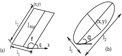
We propose two basic shape representation schemes: parallelepiped (or parallelogram in 2-D) and ellipsoid (or ellipse in 2-D). As demonstrated in Section 4, parallelograms are more appropriate to capture the shape and extent of non-local structures in protein contact maps as opposed to MBBs. Whereas ellipsoids (or ellipses) are suitable for vortices in fluid flow data as mentioned earlier. Note that the first scheme subsumes the MBB representation, and the second scheme subsumes circles. For highly irregular-shaped features such as defect structures in materials, we plan to use sampled boundary points, known as landmarks [Rao and Suryawanshi, 1996].
As shown in Figures 1(a) and 1(b), the shape descriptors of a parallelogram and an ellipse can be described as a0 ✁ ✄ ✆ ✄ ✟ ✟ ✡ ✟ ✌ ✎ ✑ ✒ ✔ ✖ ✘ ✔ ✚ ✜ ✔ ✚ ✤ ✔ ✧ ✔ ✩ ✪ and a0 ✡ ✟ ✟ ✮ ✁ ✰ ✡ ✌ ✎ ✑ ✒ ✔ ✖ ✘ ✔ ✚ ✜ ✔ ✚ ✤ ✔ ✧ ✪ , respectively. These descriptors can also be extended to 3D.
2.2 Dataset Representation
The dataset ✴ consists of ✵ features located in ✶ maps ( ✶ ✪ 1), denoted as ✷ = ✸ ✹ ✜ ✔ ✹ ✤ ✔ ✻ ✻ ✻ ✔ ✹ ✆ ✽ . The ✵ features are categorized into ✚ types, corresponding to ✚ unique labels ✾ =✸ ✿ ✜ ✔ ✿ ✤ ✔ ✻ ✻ ✻ ✔ ✿ ✟ ✽ . The categorization of features is governed by the underlying domain. A feature's geometric properties such as shape and size are captured by adopting one of the supported representation schemes. A feature ❀ thus can be described as a vector ✎ mapID, location, a0 ❁ ✡ ❃ , type ✪ , where type ❄ ✾ , mapID ❄ ✷ indicates the map where ❀ occurs, location identifies ❀ 's position within the map, and a0 ❁ ✡ ❃ ❄ ✸ a0 ✁ ✄ ✆ ✄ ✟ ✟ ✡ ✟ ✔ a0 ✡ ✟ ✟ ✮ ✁ ✰ ✡ ✽ captures the shape of ❀ .
Note that in the rest of the paper, we refer to a feature corresponding to the above vector as a spatial object. We assume the following order among the ✶ maps: ✹ ✜ ✎ ✹ ✤ ✎ ✻ ✻ ✻ ✎ ✹ ✆ . If the ✶ maps correspond to ✶ snapshots, they are ordered temporally. If they are from different datasets (e.g., different protein contact maps), the order among them is imposed by arbitrarily assigning each map a unique ID. Furthermore, the lexicographic order among the ✚ feature types is imposed as follows: ✿ ✜ ✎ ✿ ✤ ✎ ✻ ✻ ✻ ✎ ✿ ✟ .
2.3 Object-oriented Distance Metrics
The proposed algorithms use the following metrics to measure the distance between two objects ❍ ✮ and ❍ ■ located in the same map.
- ❏ Point-Point distance: This is simply the Euclidian distance between object centroids.
- ❏ Line-Line distance: If ❍ ✮ and ❍ ■ are parallelepipeds (or parallelograms), we first identify the line segment between the midpoints of the top and bottom surfaces
(or sides) in each object, then compute the shortest distance between these two line segments as the line-line distance between ❍ ✮ and ❍ ■ . We identify the top and bottom surfaces (or sides) by selecting a reference axis in the underlying Cartesian coordinate space, specifically, the ❑ -coordinate in 3D and ✖ -coordinate in 2D. If ❍ ✮ and ❍ ■ are ellipsoids (or ellipses), the line-line distance is between the two major axes.
- ❏ Boundary-Boundarydistance: This is the shortest distance between the boundaries of ❍ ✮ and ❍ ■ . When ❍ ✮ and ❍ ■ are represented as ellipses, the boundary-boundary distance is the shortest pair-wise distance between points sampled on the boundaries (or surfaces in 3D). The number of sampled points is user-specified.
Notice that the line-line and boundary-boundary metrics are able to take objects' geometric properties into account. The algorithms also support Hausdorff distance [Atallah, 1983]. Since this distance is not applicable to the applications described in this article, we do not discuss it here.
Two objects ❍ ✮ and ❍ ■ have a closeTo relationship if the distance between them is ▲ ▼ , where ▼ is a user-specified parameter. Two objects are neighbors if they have a closeTo relationship. We also define the isAbove relationship between ❍ ✮ and ❍ ■ . In a coordinate system, ❍ ✮ is said to have a isAbove relationship with ❍ ■ , if the upper-left corner of ❍ ✮ 's Minimum Bounding Box (MBB) 1 , denoted as ( ✒ ✮ ✔ ✖ ✮ ✔ ❑ ✮ ), and the upper left corner of ❍ ■ 's MBB, denoted as ( ✒ ■ ✔ ✖ ■ ✔ ❑ ■ ), meets the following condition: ✑ ❑ ✮ ✪ ❑ ■ ✘ ❖ a80 ✑ ❑ ✮ ✌ ❑ ■ ✘ ❙ a80 ✑ ✖ ✮ ✪ ✖ ■ ✘ ❖ ✑ ✑ ✖ ✮ ✌ ✖ ■ ✘ ❙ ✑ ✒ ✮ ✎ ✒ ■ ✘ ✘ ❬ ❬ in a 3-Dmap, or ✑ ✖ ✮ ✪ ✖ ■ ✘ ❖ a80 ✑ ✖ ✮ ✌ ✖ ■ ✘ ❙ ✑ ✒ ✮ ✎ ✒ ■ ✘ ❬ in a 2-Dmap.
2.4 Spatial Object Association Pattern (SOAP)
(b)
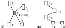
Figure 2: SOAP Types: (a)Star (b)Sequence
A Spatial Object Association Pattern (SOAP) of size ❝ , denoted as ❝ -SOAP, characterizes the closeTo relationships among ❝ object types. In this article, we focus on two types of SOAPs: Star and Sequence (Figure 2). As discussed earlier, these two SOAP types can characterize different spatial relationships among objects. These two SOAP types can be abstracted as undirected graphs, where a node corresponds to an object-type ✿ ✮ ❄ ✾ , and an edge ✑ ✿ ✮ ✔ ✿ ■ ✘ indicates that ✿ ✮ and ✿ ■ are required to have a closeTo relationship.
- ❏ Star SOAPs (Figure 2a) have a center object-type, which is required to have a closeTo relationship with all the other object-types in the same SOAP.
- ❏ Sequence SOAPs (Figure 2b) of size ❝ ❞ =( ✿ ❡ ✮ ❢ : ❣ ❄ [1, ❝ ]) satisfy two constraints, where ✿ ❡ ✮ ❢ is the ❣ ❤ ✐ element in ❞ : (1) closeTo( ✿ ❡ ✮ ❢ ✔ ✿ ❡ ✮ ❥ ✜ ❢ )=true and (2) isAbove( ✿ ❡ ✮ ❢ ✔ ✿ ❡ ✮ ❥ ✜ ❢ )=true, where 1 ▲ i ▲ k-1. Sequence SOAPs are mainly motivated by our observation on protein contact maps, where non-local structures, i.e, features, tend to line up in a Sequence like manner.
1 For a 3DMBB, it is the upper-left corner of its top surface.
These two SOAP types can also be represented as lists. Let ✿ a0 ✂ ❤ ✆ be the center of a star ❝ -SOAP ❞ , and ✸ ✿ ❡ ✮ ❢ : ❣ ❄ [1,❝ - 1] ✽ be the other k-1 object-types in ❞ , where ✿ ❡ ✜ ❢ ▲ ✻ ✻ ✻ ▲ ✿ ❡ ☎ ✆ ✜ ❢ . SOAP ❞ can then be described by the list ❞ =(✿ a0 ✂ ❤ ✆ , ✿ ❡ ✜ ❢ ✔ ✻ ✻ ✻ ✔ ✿ ❡ ☎ ✆ ✜ ❢ ), where closeTo( ✿ a0 ✂ ❤ ✆ ✔ ✿ ❡ ✮ ❢ )=true ( ❣ ❄ [1, ❝ -1]). Whereas elements in a sequence SOAP correspond to a list by definition and cannot be forced into lexicographical order. For instance, the two sequence SOAPs ✑ a0 ✞ ✠ ✘ and ✑ a0 ✠ ✞ ✘ are different.
A SOAP is autocorrelated if an object-type occurs multiple times. For example, ✑ ✿ ✜ ✔ ✿ ✜ ✔ ✿ ✤ ✘ is an autocorrelated 3SOAP, where ✿ ✜ occurs twice. An instance of a SOAP ❞ is the set of objects that meet all the requirements specified by ❞ , including those on object-types and closeTo (or isAbove) relationships.
We define two measures-support and realization- to characterize the importance of a SOAP. The support of a SOAP ❞ is the number of maps in the dataset where ❞ occurs. Assume support(p)=s, let ✵ ✮ be the number of ❞ 's instances in the ❣ ❤ ✐ map where ❞ appears, realization( ❞ )=min ✸ ✵ ✮ ✽ . A pattern ❞ is frequent if support(❞ ) ✌ minSupp, and prevalent if realization(❞ ) ✌ minRealization, where minSupp and minRealization are user-specified parameters.
3 Algorithms 3.1 Data Organization
We organize ✴ in the following manner. The ✵ objects are first grouped into ✚ partitions, where each partition is composed of objects of the same type. Within each partition, objects are ordered by their map IDs and locations in a map. This data organization is analogous to the format used for association rule mining [Zaki et al., 1997]. Note that each object can be uniquely identified by combining the following information: mapID, label, and locationID in the map.
3.2 Equivalence Classes
Based on the list-based SOAP representation (Section 2.4), we organize SOAPs into equivalence classes. A ❝ - equivalence class, denoted as ❝ -EquiClass, is defined as the set of ❝ -SOAPs that (i) are of the same SOAP type, and (ii) have the same prefix, where the prefix of a ❝ -SOAP is its first k-1 elements. By using equivalence classes, our mining algorithms only need to compute the closeTo or isAbove relationships between objects once. The equivalence classes also help to improve the memory locality of the algorithms, which result in significant performance gains. Moreover, equivalence classes also enable the algorithms to smoothly scale to large datasets [Zaki et al., 1997].
The next two sections describe the algorithms that discover Star and Sequence SOAPs. For each frequent SOAP, the algorithms store information about all of its instances. Such information allows the algorithms to locate every object involved in an instance.
3.3 Mining Star SOAPs
Figure 3 outlines the algorithm that discovers star SOAPs. The first step generates frequent 1-SOAPs (line 1). For each object-type ✿ ✮ , the procedure gen1SOAPcounts the number of maps that contain at least one object of type ✿ ✮ . If the count
✌ minSupp, then ❞ ✜ =( ✿ ✮ ) is a frequent 1-SOAP. The set of all frequent 1-SOAPs is denoted by ✍ ✜ .
The next step, gen2EquiClass, discovers 2-SOAPs and organizes them into 2-EquiClasses (line 2). The pseudo-code of gen2EquiClass is described in Figure 4. A 2-EquiClass is generated for each frequent 1-SOAP (Figure 4:line 2). The 2-EquiClass of 1-SOAP (✿ ✮ ) ❄ ✍ ✜ , denoted by ✏ ✤ ✑ a0 ✒ , contains frequent 2-SOAPs in the form of ( ✿ ✮ ✔ a0 ). To generate ✏ ✤ ✑ a0 ✒ , the procedure considers the following 2-SOAPs as candidates: (✿ ✮ ✔ ✿ ■ ), where (✿ ■ ) ❄ ✍ ✜ (Figure 4:line 3). For each candidate 2-SOAP ❞ ✤ =(✿ ✮ ✔ ✿ ■ ), the procedure identifies all the maps where ❞ ✤ occurs (Figure 4:lines 6-11). An instance of ❞ ✤ =(✿ ✮ ✔ ✿ ■ ) is an object pair ✑ ❍ ✮ ✔ ❍ ■ ✘ , where (❍ ✮ ✻ ✔ ✖ ❞ ✕ =✿ ✮ ) ❙ ✑ ❍ ■ ✻ ✔ ✖ ❞ ✕ =✿ ■ ) ❙ (distance(❍ ✮ ✔ ❍ ■ ,distType) ▲ ▼ ). If ❞ ✤ occurs in ✌ minSupp maps, then it is frequent and is added to ✏ ✤ ✑ a0 ✒ (Figure 4:line 12).
Algorithmmine starSOAP( ✘ ,minSupp, minRealization, distType, ✙ ) 1. ✚ ✛ ✢ gen1SOAP(); // 1-SOAPs 2. ✣ ✤ ✦ ✢ gen2EquiClass( ✘ ✑ ✚ ✛ , star, parList); //parList: parameters 3. ☎ ✢ ✤ ; 4. while (1) ★ 5. ✣ ✤ ✩ ✪ ✛ ✢ ✬ ; //the set of (k+1)-EquiClasses 6. foreach ☎ -EquiClass ✣ ✩ ✮ ✣ ✤ ✩ 7. foreach ☎ -SOAP ✁ ✩ ✰ ✒ ✮ ✣ ✩ 8. ✣ ✩ ✪ ✛ ✢ ✬ ; // the prefix of ✣ ✩ ✪ ✛ is ✁ ✩ ✰ ✒ 9. foreach ☎ -SOAP ( ✁ ✩ ✰ ✵ ✮ ✣ ✩ ✷ ✸ ✺ ✮ ✼ ■ ✷ 10. ✁ ✩ ✪ ✛ ✢ append( ✁ ✩ ✰ ✒ , lastElement( ✁ ✩ ✰ ✵ ) ); 11. ✾ ✿ ✩ ✪ ✛ ✢ ★ ❀ ✒ ❁ ❀ ✒ contains ✁ ✩ ✰ ✒ and ✁ ✩ ✰ ✵ ❃ ; 12. foreach ❀ ✒ ✮ ✾ ✿ ✩ ✪ ✛ 13. if ( countStarInstances( ❀ ✒ ✑ ✁ ✒ ✑ ✁ ✵ ) ❅ 1) mapCnt++; 14. if ( mapCnt ❅ ❀ ✮ ✂ ❇ ❉ ✁ ✁ ) ✣ ✩ ✪ ✛ ✢ ✣ ✩ ✪ ✛ ❋ ★ ✁ ✩ ✪ ✛ ❃ ; 15. if ✺ ✣ ✩ ✪ ✛ ● ❍ ✬ ✷ ✣ ✤ ✩ ✪ ✛ ✢ ✣ ✤ ✩ ✪ ✛ ❋ ✣ ✩ ✪ ✛ ; 16. if (minRealization ❏ 1) markPrevFreqSOAPs( ✣ ✩ ✪ ✛ ); 17. if ( ✣ ✤ ✩ ✪ ✛ ❍ ✬ ) return; //terminate 18. k++; //increase SOAP size ❃ //while(1)The algorithm next discovers SOAPs of size ✪ 2 (Figure 3:lines 4-17 ). Two ❝ -SOAPs in the same ❝ -EquiClass are combined to construct a candidate (❝ +1)-SOAP. For each candidate (❝ +1)-SOAP ❞ ☎ ❥ ✜ derived by appending the last element of ❞ ☎ ✑ ■ to ❞ ☎ ✑ ✮ (Figure 3: line 10), the algorithm identifies all the maps where ❞ ☎ ❥ ✜ occurs (Figure 3:lines 11-14). (The ❣ ❤ ✐ k-SOAP in a k-EquiClass is denoted as ❞ ☎ ✑ ✮ .) The procedure countStarInstances( ✹ ✮ ✔ ❞ ☎ ✑ ✮ ✔ ❞ ☎ ✑ ■ ) (Figure 3:line 13) computes the instances of ❞ ☎ ❥ ✜ in map ✹ ✮ by combining instances of ❞ ☎ ✑ ✮ and ❞ ☎ ✑ ■ . Two instances from ❞ ☎ ✑ ✮ and ❞ ☎ ✑ ■ are joined to produce a ❞ ☎ ❥ ✜ instance if they have the same first ❝ -1 objects and different last object. SOAPs with the same prefix are organized into one equivalence class as they are being generated (see Figure 3:lines 5, 8, 14, 15). The mining process stops when all the frequent SOAPs have been discovered (Figure 3:line 17).
To discover frequent SOAPs, the algorithm only needs to consider a SOAP's presence in a map (Figure 3:line 13). Hence, some of the discovered frequent SOAPs may not be prevalent if minRealization ✪ 1. In this case, the procedure markPrevFreqSOAPs is called to identify the SOAPs that are both prevalent and frequent (Figure 3:line 16). It is necessary to keep SOAPs that are frequent but not prevalent. We explain this by a simple example. Let ✸ ❑ ✜ ✔ ▲ ✜ ✔ ▲ ✤ ✽ be the three neighboring objects in a map and minRealization=2. To derive the two instances of SOAP (❑ ✔ ▲ ), ✑ ❑ ✜ ✔ ▲ ✜ ✘ and ✑ ❑ ✜ ✔ ▲ ✤ ✘ ,
Algorithm gen2EquiClass ( ✘ ✑ ✚ ✛ ✑ ✰ ❃ ✄ ✁ a0 ✂ ✁ ✡ ,parList ) //✚ ✛ :freq. 1-SOAPs 1.✣ ✤ ✦ ✢ ✬ ; //the set of 2-EquiClasses 2.foreach ( a0 ✒ ) ✮ ✚ ✛ 3. ✣ ✦ ✰ ☎ ✒ ✢ ✬ //2-EquiClass with prefix of a0 ✒ ; 4. foreach ( a0 ✵ ) ✮ ✚ ✛ 5. ✁ ✦ ✢ ( a0 ✒ ✑ a0 ✵ ); //a candidate 6. ✾ ✿ ✦ ✢ ★ ❀ ✒ ❁ ✺ ❀ ✒ contains a0 ✒ and a0 ✵ ) ❃ ; 7. foreach ❀ ✒ ✮ ✾ ✿ ✦ 8. foreach ✺ ❃ ✒ ✑ ❃ ✵ ✷ ✮ ❀ ✒ ❁ ✺ ❃ ✒ ✆ ✟ ✄ ✞ ✡ ✟ ❍ a0 ✒ ✷ ✸ ✺ ❃ ✵ ✆ ✟ ✄ ✞ ✡ ✟ ❍ a0 ✵ ✷ 9. if ( (soapType=Sequence) ✸ (✠ isAbove ✺ ❃ ✒ ✑ ❃ ✵ ✷ ✷ ) continue; 10. if distance( ❃ ✒ ✑ ❃ ✵ , distType) ✼ ✙ ) addInstance( ✁ ✦ ✑ ✺ ❃ ✒ ✑ ❃ ✵ ✷ ); 11. if ( cntInst( ✁ ✦ ✑ ❀ ✒ ✷ ❅ 1) mapCnt++; 12. if ( mapCnt ❅ minSupp ) ✣ ✦ ✰ ☎ ✒ ✢ ✣ ✦ ✰ ☎ ✒ ❋ ★ ✁ ✦ ❃ ; 13.if ( ✣ ✦ ✰ ☎ ✒ ● ❍ ✬ ) ✣ ✤ ✦ ✢ ✣ ✤ ✦ ❋ ✣ ✦ ✰ ☎ ✒ ;the 1-SOAP ( ❑ ) must be maintained even though its realization is 1 ( ✎ ✡ ) in the map.
Correctness: It is straightforward to show that the algorithm discovers all the frequent 1-SOAPs and 2-SOAPs. Thus to prove the algorithm is correct, we only need to show that every frequent ❝ -SOAP (❝ ✪ 2) will be considered as a candidate. Assume ❞ ☎ =(✿ ❡ ✜ ❢ ✔ ✻ ✻ ✻ ✔ ✿ ❡ ☎ ✆ ✤ ❢ ✔ ✿ ❡ ☎ ✆ ✜ ❢ ✔ ✿ ❡ ☎ ❢ ) is frequent, then the two (k-1)-SOAPs ❞ ☎ ✆ ✜ ✑ ✮ = ( ✿ ❡ ✜ ❢ ✔ ✻ ✻ ✻ ✔ ✿ ❡ ☎ ✆ ✤ ❢ ✔ ✿ ❡ ☎ ✆ ✜ ❢ ) and ❞ ☎ ✆ ✜ ✑ ■ = ( ✿ ❡ ✜ ❢ ✔ ✻ ✻ ✻ ✔ ✿ ❡ ☎ ✆ ✤ ❢ ✔ ✿ ❡ ☎ ❢ ) must also be frequent and in the same equivalence class. Thus the algorithm will consider ❞ ☎ as a candidate. It is trivial to show that the procedure countStarInstances identifies all the instances of a candidate SOAP. ☞
3.4 Mining Sequence SOAPs
The pseudo-code is given in Figure 5. Unlike mining Star SOAPs, which uses two k-SOAPs in the same equivalence class to generate a candidate (k+1)-SOAP (❝ ✌ 2), the algorithm joins one ❝ -SOAP and one 2-SOAP.
The first two steps (lines 1-2) discover all the frequent 1SOAPs and 2-SOAPs. The isAbove relationship is checked by the procedure isAbove(❍ ✮ ✔ ❍ ■ ) (Figure 4:line 9). For each ❝ -SOAP ❞ ☎ =( ✿ ❡ ✜ ❢ ✔ ✻ ✻ ✻ ✔ ✿ ❡ ☎ ❢ ), the algorithm first locates the 2EquiClass ✏ ✤ ✑ a0 ✌ ✩ ✎ , in which every 2-SOAP is in the form (✿ ❡ ☎ ❢ ✔ ✿ ❡ ■ ❢ ):closeTo(✿ ❡ ☎ ❢ ✔ ✿ ❡ ■ ❢ ) ❙ isAbove(✿ ❡ ☎ ❢ ✔ ✿ ❡ ■ ❢ ) (line 7). A set of candidate (k+1)-SOAPs are then generated by combining ❞ ☎ with each 2-SOAP in ✏ ✤ ✑ a0 ✌ ✩ ✎ (lines 8-9). Same as mining Star SOAPs, a candidate (k+1)-SOAP ❞ ☎ ❥ ✜ is frequent if it appears in ✌ minSupp maps (lines 10-13). The procedure countSeqInstances( ✹ ✮ ✔ ❞ ☎ ✑ ✮ ✔ ❞ ✤ ✑ ■ ) (line 12) identifies instances of ❞ ☎ ❥ ✜ in map ✹ ✮ , where ❞ ☎ ❥ ✜ is a candidate SOAP based on ❞ ☎ ✑ ✮ and ❞ ✤ ✑ ■ . Two instances ✑ ☎ ✑ ✮ and ✑ ✤ ✑ ■ , from ❞ ☎ ✑ ✮ and ❞ ✤ ✑ ■ respectively, are combined to produce an instance of ❞ ☎ ❥ ✜ if the last object in ✑ ☎ ✑ ✮ is the same as the first object in ✑ ✤ ✑ ■ . For the same reason explained before, the algorithm calls the procedure markPrevFreqSOAPs to label SOAPs being bothprevalent and frequent if minRealization ✪ 1 (line 15). The algorithm stops when no more SOAPs can be discovered (line 14).
Correctness: For each frequent sequence k-SOAP ❞ ☎ =( ✿ ❡ ✜ ❢ ✔ ✻ ✻ ✻ ✔ ✿ ❡ ☎ ✆ ✜ ❢ ✔ ✿ ❡ ☎ ❢ ✘ , the following two SOAPs must also be frequent: ❞ ☎ ✆ ✜ =(✿ ❡ ✜ ❢ ✔ ✻ ✻ ✻ ✔ ✿ ❡ ☎ ✆ ✜ ❢ ) and ❞ ✤ =(✿ ❡ ☎ ✆ ✜ ❢ ✔ ✿ ❡ ☎ ❢ ). Thus, ❞ ☎ will be considered as a candidate and be discovered. It is trivial to show that the procedure countSeqInstances identifies all the instances of a candidate SOAP. ☞
Algorithmmine sequenceSOAP( ✘ ,minSupp, minRealization, distType, ✙ ) 1. ✚ ✛ ✢ gen1SOAP(); 2. ✣ ✤ ✦ ✺ ❃ ✆ ✚ ✦ ✷ ✢ gen2EquiClass(✘ ✑ ✚ ✛ , Sequence, parList);//parList:parameters 3. ☎ ✢ ✤ ; 4. while (1) ★ 5. ✚ ✩ ✪ ✛ ✢ ✬ ; //initialize the set of ✺ ☎ ❥ ✜ ✷ -SOAPs; 6. foreach SOAP ✁ ✩ ✰ ✒ ❍ ✒ a0 ✌ ✔ ✎ ✑ ✆ ✆ ✆ ✑ a0 ✌ ✩ ✖ ✛ ✎ ❏ ✮ ✚ ✩ 7. ✣ ✦ ✰ ☎ ✌ ✩ ✎ ✢ ✣ ✦ ✰ ☎ ✌ ✩ ✎ ✮ ✣ ✤ ✦ ✷ ✸ ✺ ✣ ✦ ✰ ☎ ✌ ✩ ✎ ✆ ✁ ✆ ✡ ✘ ✮ ✙ ❍ a0 ✌ ✩ ✎ ✷ ; 8. foreach 2-SOAP ✁ ✦ ✰ ✵ ✮ ✣ ✦ ✰ ☎ ✌ ✩ ✎ 9. ✁ ✩ ✪ ✛ ✢ append( ✁ ✩ ✰ ✒ , lastElement( ✁ ✦ ✰ ✵ ) ); 10. ✾ ✿ ✩ ✪ ✛ ✢ ★ ❀ ✒ ❁ ❀ ✒ contains both ✁ ✩ ✰ ✒ and ✁ ✦ ✰ ✵ ❃ ; 11. foreach ❀ ✒ ✮ ✾ ✿ ✩ ✪ ✛ 12. if ( countSeqInstances( ❀ ✒ ✑ ✁ ✩ ✰ ✒ ✑ ✁ ✦ ✰ ✵ ✷ ❅ 1) mapCnt++; 13. if ( mapCnt ❅ minSupp ) ✚ ✩ ✪ ✛ ✢ ✚ ✩ ✪ ✛ ❋ ★ ✁ ✩ ✪ ✛ ❃ ; 14. if ( ✚ ✩ ✪ ✛ ❍ ✬ ) return; //terminate the process; 15. if (minRealization ❏ 1) markPrevFreqSOAPs( ✚ ✩ ✪ ✛ ); 16. k++; //increase SOAP size ❃ //while(1)Other SOAP types can also be defined. For instance, we can define Clique SOAPs, which require every pair of objects in the same SOAP have a closeTo relationship. We can also define SOAPs that involve other types of spatial relations such as topological relations.
4 Experimental Evaluation
In this section, we evaluate the algorithms on a protein contact map dataset. We start with a brief description on the dataset generation process and the domain-specific usefulness measurement adopted in this work. We then present results to analyze the impact from different distance metrics and SOAP types. Finally, we present performance characterization of the algorithms.
4.1 Data Preprocessing and Representation
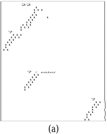
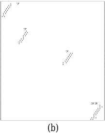
We first generate contact maps for ✛ ✔ ✜ ✣ ✡ proteins taken from the Protein Data Bank [Berman et al., 2000]. For a protein with N amino acids, its contact map ✠ is a ✦ ✧ ✦ binarymatrix. The position ✠ (❣ ✔ ✪ ) is set to 1 if the distance between the ❣ ❤ ✐ and ✪ ❤ ✐ residues is less than a threshold and 0 otherwise [Vendruscolo and Domany, 1997]. We use 6 ˚A as the threshold as suggested in the literature [Zaki, 2002]. We then extract features in contact maps. A contact map feature is composed of a set of positions, where each position and at least one of its eight neighbors contain a '1' (see Figure 6 for examples). We apply a simple region growing approach to extract features in contact maps [Yang et al., 2004]. We then use an entropy-based clustering algorithm to cluster features into ✚ groups (or classes) [Cheng et al., 1999]. Features in a class have similar geometric properties such as shape and extent.
A total of ✬ ✔ ✭ ✭ ✰ ✔ ✜ ✱ ✱ features are extracted from the ✛ ✔ ✜ ✣ ✡ contact maps. These features are clustered into ✡ ✛ classes. The average number of features in each map is about ✬ ✬ ✱ . Many of these features correspond to well-known protein secondary structures and are also validated by domain experts. We represent each feature by its minimum bounding parallelogram and label the parallelogram by the feature's class ID.
4.2 Domain Specific Usefulness Measurement
The structure of a protein often provides information about its functionality. Thus, one can predict a protein's function based on the function of other structurally similar proteins.
Frequent SOAPs in contact maps characterize proteins' structure. They can be used to generate signatures for different proteins. For instance, the SOAP (7 7 7 22), which is automatically discovered by our algorithms as both Star and Sequence, can be used to identify the following structurally and functionally similar a0 -proteins: 1h3t, 1h3u and 1h3v (IDs from PDB). (See Figures 6(a) and 6(b) for an illustration of these SOAPs.)
However, a SOAP is unlikely to add any value to the signature, if it is randomly associated with proteins of different classes. To prune away such SOAPs, we use an entropy-based approach. For a given SOAP, we first identify its associated proteins. We then compute the SOAP's entropy by integrating the proteins' lineage information from the database of Structural Classification of Proteins (SCOP) 2 . A protein's SCOP lineage is organized into 6 hierarchical levels according to its structure. We look at the first two levels: ✁ ✜ :✿ ✚ ❑ ✂ ✂ , and ✁ ✤ :❀ ❍ ✚ ✆ . ✁ ✜ consists of 11 classes such as ✞ -protein, a0 - protein, and small protein. ✁ ✤ further divides proteins into sub-classes based on proteins' folding structures. Let ✦ be the number of proteins whose contact maps contain the SOAP ❞ , and ✵ ✮ be the number of proteins among these ✦ proteins in the ❣ ❤ ✐ class, the entropy of ❞ at the first SCOP level is then computed as: ✟ ✑ ❞ ✘ ✌ ✠ ✜ ✜ ✮ ❍ ✜ ☛ ✑ ✵ ✮ ✌ ✦ ✘ ✧ ✚ ❍ ✎ ✤ ✑ ✵ ✮ ✌ ✦ ✘ [Shannon, 2001]. ✟ ✑ ❞ ✘ essentially measures how well ❞ 's associated proteins distribute among different proteins classes. In our experiments, we observe that SOAPs with entropy ▲ 2.0 show good quality and can be used to generate signatures. This observation is also validated by domain experts.
For each SOAP with entropy ▲ 2.0, we next identify the protein class that dominates its associated proteins. For example, the dominating protein class of the clique SOAP (5 7 7 22) is a0 -protein, as ✬ ✰ ✬ out of its ✡ ✬ ✱ associated proteins are a0 -proteins. As suggested by domain experts, we would like to have many SOAPs for a certain protein class. A large number of SOAPs not only cover a wide range of proteins, but can also be used to identify structurally similar proteins from different aspects. This criterion is used to evaluate the discovered SOAPs. Note that even if two SOAPs have the same dominating protein class, their associated proteins can be very different.
2 http://scop.mrc-lmb.cam.ac.uk/scop/
4.3 Impact of Distance Metrics
Due to lack of space, we only report the results produced from the following parameter setting: minSupp=✬ %, minRealization= ✬ , and ▼ = ✱ ✱ ˚A.
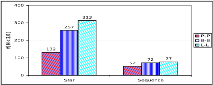
Figure 7 shows the impact of the three distance metrics on different SOAP types. One can observe that the Line-Line (L-L) distance generates the most number of SOAPs for both SOAP types, whereas the Point-Point (P-P) distance the least. This is expected as the P-P distance does not consider the shape and size of spatial objects, in contrast with the other two. One may argue that more SOAPs can be identified by increasing the distance threshold in the case of P-P distance. However, it is very difficult to find an appropriate threshold value, as the size of a feature, i.e., the number of bit- ✬ positions, varies drastically, from ✡ up to several thousand.
The advantage of using L-L and B-B distance metrics becomes more significant when looking at the SOAPs' dominating protein classes. Tables 1-3 summarize the number of SOAPs in major protein classes. One can see that, if the P-P distance is used (Table 1), only ✣ ✬ SOAPs are discovered in small proteins as against ✬ ✣ ✣ SOAPs in a0 -proteins. On the other hand, SOAPs based on L-L or B-B distance show a relatively more balanced behavior(Tables 2-3). Compared with P-P distance, much more SOAPs in a0 -proteins or small proteins are discovered. For instance, in the L-L case (Table 2), there are ✬ ✛ ✭ and ✡ ✭ ✣ SOAPs are identified in a0 -proteins and small proteins respectively. Also the B-B distance produces the most number ( ✬ ✑ ) of SOAPs for ✞ -proteins (Table 3).
The differences exhibited by SOAPs from different distance metrics show that it is important for our algorithms to support multiple distance metrics, especially metrics which consider objects' extent.
| Type | #(✓ ) | #(✔ ) | #(small) | #(peptide) |
|---|---|---|---|---|
| Star | 2 | 103 | 19 | 7 |
| Sequence | 4 | 30 | 12 | 4 |
| Total | 6 | 133 | 31 | 11 |
| Type | #(✓ ) | #(✔ ) | #(small) | #(peptide) |
|---|---|---|---|---|
| Star | 1 | 133 | 167 | 12 |
| Sequence | 4 | 37 | 36 | 6 |
| Total | 5 | 170 | 203 | 18 |
4.4 Impact of SOAP Types
As we move down to the second SCOP lineage level, ✁ ✤ : ❀ ❍ ✚ ✆ , we discover that different types of SOAPs can actually distinguish different protein folding structures. Proteins in the same class (e.g., a0 -protein) are further classified into structurally similar sub-groups according to their folding structures. Table 4 lists the a0 -protein folds that are distinguished by each SOAP type, where SOAPs are generated based on the L-L distance. The folds in bold are those that are associated with only one SOAP type. Whereas other folds in the table are distinguished by two or more SOAP types. Folds in other protein classes show a similar trend. For example, the ✞ -protein fold "Cyclin-like" is only associated with sequence SOAPs.
| Type | #(✓ ) | #(✔ ) | #(small) | #(peptide) |
|---|---|---|---|---|
| Star | 8 | 145 | 91 | 13 |
| Seq. | 6 | 40 | 25 | 6 |
| Total | 14 | 185 | 116 | 19 |
The above results can potentially help domain experts address some important biological issues, for instance, predicting a protein's function based on the SOAPs contained in its contact map.
| Star | Immunoglobulin-like beta-sandwich Concanavalin A-like lectins/glucanases Trypsin-like serine proteases Cupredoxin-like Acid proteases Cysteine proteinases |
| Sequence | Immunoglobulin-like beta-sandwich Concanavalin A-like lectins/glucanases Trypsin-like serine proteases Lipocalins Nucleoplasmin-like/VP |
| Type | minSupp=2% | minSupp=1% |
|---|---|---|
| Star | 15.54 | 21.53 |
| Sequence | 4.83 | 7.79 |
4.5 Running Time
Table 5 shows the time taken to discover the two types of SOAPs at two minSupp values. All the experiments were carried out on a Pentium ✬ ✻ ✜ GHz computer of ✡ ✱ a0 MB main memory. To discover SOAPs in ✛ ✔ ✜ ✣ ✡ protein contact maps containing ✬ ✔ ✭ ✭ ✰ ✔ ✜ ✱ ✱ objects, the algorithms take about ✡ ✭ seconds when minSupp= ✡ ✂ and about ✣ ✭ seconds when minSupp= ✬ ✂ . Although running time increases as minSupp decreases, the algorithm scales very well. We attribute this good performance to the use of equivalence classes.
5 Conclusion and OngoingWork
In this paper, we present a general framework to uncover two types of spatial association patterns among features in scientific data. The framework represents features as spatial objects instead of points. It also supports multiple distance metrics. Empirical results on protein contact maps show that the framework is both efficient and scalable. Furthermore, the discovered SOAPs are meaningful and can potentially be used to address important biological issues.
The SOAP mining problem in this article shares some similarity with frequent subgraph mining [Yan and Han, 2002]. In order to apply the conventional graph mining algorithms for SOAP mining, the notion of nodes needs to be extended to integrate spatial properties such as location and shape. Also, the notion of edge needs to be modified to reflect different spatial relationships such as closeTo.
We are currently extending the framework in several directions. First, we are examining other shape representation schemes such as the landmark-based approach for highly irregularly shaped features. Second, we are evaluating other types of object association patterns, for example, clique SOAPs, where each object has a closeTo relationship with every other object in the same SOAP. Third, we are interested in evaluating the algorithms on datasets from other scientific domains, including molecular dynamics and fluid flow dynamics. Some of our ongoing work is reported in a technical report [Yang et al., 2005]. Finally, we are investigating potential approaches towards association based spatio-temporal reasoning.
Acknowledgments: We thank D. Polshakov and K. Marsolo for helping us validate the experimental results, and thank Dr. J. Wilkins and Dr. R. Machiraju for valuable comments on the initial ideas.
@inproceedings{ijcai2005p177,
  title     = {Mining Spatial Object Associations for Scientific Data},
  author    = {Yang, Hui and Parthasarathy, Srinivasan and Mehta, Sameep},
  booktitle = {Proceedings of the Nineteenth International Joint Conference on
               Artificial Intelligence, {IJCAI-05}},
  publisher = {International Joint Conferences on Artificial Intelligence},
  editor    = {Leslie Pack Kaelbling and Alessandro Saffiotti},
  pages     = {902--906},
  year      = {2005},
  url       = {https://ijcai.org/proceedings/2005/177},
}
TY - CPAPER TI - Mining Spatial Object Associations for Scientific Data AU - Yang, Hui AU - Parthasarathy, Srinivasan AU - Mehta, Sameep T2 - Proceedings of the Nineteenth International Joint Conference on Artificial Intelligence, IJCAI-05 PB - International Joint Conferences on Artificial Intelligence PY - 2005 SP - 902 EP - 906 UR - https://ijcai.org/proceedings/2005/177 ER -Copied
Machine-readable versions of this paper, for tools and AI agents:





