Fast and Complete Symbolic Plan Recognition

1 Introduction

vations may be of continuous actions, maintained over time. For instance, an observation of a soccer player may include its team name, uniform number, current position, velocity, etc. The computational cost of matching such observations against all possible plan-steps is non-trivial, and grows in the complexity of the observation tuple. However, existing investigations ignore this cost. Second, with few exceptions, existing algorithms focus on the current state query (e.g.,[Tambe and Rosenbloom, 1995; Bui, 2003]). Some go as far as to ignore all [Tambe and Rosenbloom, 1995] or portions [Wærn and Stenborg, 1995] of the observation history, and are unable to utilize negative evidence (where an expected action was not observed).

Plan recognition is the process of inferring another agent's plans, based on observations of its interaction with its environment. Recent applications of plan recognition require observing agents whose behavior is reactive [Rao, 1994], in that the observed agent may interrupt plan execution, switch to a different plan, etc. Such applications include intrusion detection applications [Geib and Harp, 2004], virtual training environments [Tambe and Rosenbloom, 1995], and visual monitoring [Bui, 2003].

In general, plan recognition relies on a plan library of plans potentially executed by the observed agent. Typically, the plan library is composed of top-level plans that are hierarchically decomposed. The recognizer matches observations to specific plan steps in the library. It may then infer answers to plan recognition queries, such as the currently selected top-level plans (current state query), or the ordered sequence of (completed or interrupted) selected plans (state history query).

Existing work leaves several challenges open (see Section 2 for details). First, most existing work assumes observations to be of atomic instantaneous actions. However, observations in recent applications are often complex multi-featured tuples, involving symbolic, discrete, and continuous components (e.g., multiple actuators of the agent). Moreover, obser- This paper focuses on a set of efficient algorithms that tackle these challenges: First, we develop a method for automatically generating a matching decision-tree that efficiently matches multi-feature observations, to the plan library. Second, we provide algorithms for efficiently answering the current state and state history queries. These lazy-commitment algorithms avoid computation of hypotheses on every step (as other algorithms do [Geib and Harp, 2004]). Instead, they use linear-time (current state) and polynomial-time (state-history) bookkeeping with every observation, which allows extraction of hypotheses only as needed. Our algorithms are complete, in that they admit all recognition hypotheses consistent with the history of observations; they are symbolic in that they provide hypotheses with no ranking (probabilistic or otherwise).

We explore the performance of the recognition algorithms with simulated data, and show that they are significantly faster than previous techniques. Their efficiency and completeness make them particularly suited for hybrid plan recognition approaches (e.g., [Geib and Harp, 2004]) in which a symbolic recognizer filters inconsistent hypotheses, passing them to a probabilistic inference engine.

2 Background and RelatedWork

We focus this brief discussion on closely related work, particularly allowing recognition of interruptible plans. See [Carrbery, 2001] for a recent survey of general plan recognition.

Several investigations have utilized multi-featured observations (also of continuous actions), but did not address the efficiency of matching observations to the plan library, in contrast to our work: RESC [Tambe and Rosenbloom, 1995] and RESL [Kaminka and Tambe, 2000] use a hierarchical representation (similar to what we use) to maintain a single hypothesis (RESC) or multiple hypotheses (RESL) as to the current state of an observed agent. Both algorithms ignore observation history in the current state hypotheses, and do not address state history, in contrast to our algorithms.

Geib et al. [Geib and Harp, 2004] developed PHATT, a hybrid recognizer, where a symbolic algorithm filters inconsistent hypotheses before they are considered probabilistically. PHATT assumes instantaneous, atomic actions, and takes a generate-and-test approach: With each observation, the symbolic algorithm generates a pending set of possible expected observations, which are matched against the next observation to maintain correct state history hypotheses. The size of the pending set may grow exponentially [Geib, 2004]. In contrast, our work decouples the current state and state history queries, and incrementally maintains hypotheses implicitly, without predicting impending observations. The hypotheses are thus computed only when needed (when hopefully, many of them have been ruled out).

Other investigations assume atomic observations, and do not consider the cost of matching. [Wærn and Stenborg, 1995] explores plan-recognition with limited observation history, to facilitate recognition of reactive behavior. [RetzSchmidt, 1991] develops an approach based on matching subgraphs of the plan library. However, the approach does not allow for interruptions of plans.

Our work differs significantly from probabilistic approaches, though it complements them in principle (as demonstrated by Geib et al.). [Bui, 2003] explores probabilistic reactive recognition extending hidden Markov models, focusing on current state query. [Pynadath and Wellman, 2000] explores a probabilistic grammar representation for efficient plan-recognition. None of these considers the cost of matching observations, nor separation of state history from current state queries.

3 Matching Observations to the Plan Library

As commonly done in plan recognition work (e.g., [Bui, 2003]), we utilize a hierarchical representation of the plan library (Section 3.1). We present a method for efficiently matching multi-feature observations to the library (3.2).

3.1 The Plan Library

We represent the plan library as a single-root directed acyclic connected graph, where vertices denote plan steps, and edges can be of two types: vertical edges decompose plan steps into sub-steps, and sequential edges specify the expected temporal order of execution. For the discussion, we refer to the children of the root node as top-level plans, and to all other nodes simply as plans. However, we use the term plan here in its general sense, inclusive of reaction plans, behaviors, and recipes. Indeed, to represent behavior-based agents (where typically behaviors execute over a number of time-steps), plans may have a sequential self-cycle, to allow them to be re-selected. However, no cycles are allowed hierarchically.

Each plan has an associated set of conditions on observable features of the agent and its actions. When these conditions hold, the observations are said to match the plan. For example, a kick-ball-to-goal plan (of a robotic soccer player) may have the following features: The ball must be visible, the distance to the ball is within a given range, and the opponent goal is visible within shooting distance. If all the above conditions are satisfied, the plan matches the observation.

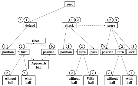
At any given time, the observed agent is assumed to be executing a plan decomposition path, root-to-leaf through decomposition edges. Figure 1 shows an example portion of a plan library, inspired by the behavior hierarchies of RoboCup soccer teams (e.g. [Kaminka and Tambe, 2000]). The figure shows decomposition edges (solid arrows) and sequential edges (dashed arrows). The top level plans are defend, attack, and score. The figure does not show the observation conditions associated with plan steps. For presentation clarity, we show the decomposition edges only to the first (in temporal order) child plans. Thus in the figure, the path root → defend → turn → with ball can be an hypothesis as to the current plan of an observed player. In realistic settings, likely more than one path will match an observation tuple, and this may result in a set of such decomposition paths, i.e., a set of hypotheses as to the current state of the observed agent (answering a current state query).

An observed agent is assumed to change its internal state in two ways. First, it may follow a sequential edge to the next plan step. Second, it may reactively interrupt plan execution at any time, and select a new (first) plan. For instance, suppose the agent was executing root → defend → turn → with ball, and then interrupted execution of this plan. It may now choose root → attack → pass, but not root → attack → turn → withball.

3.2 Efficient Matching

The first phase of recognition, common to all recognition approaches, matches the observations made by the recognizer to plans in the plan library. In contrast with previous work, we consider complex observations, that consist of a tuple of observed features, including states of the world that pertain to the agent (e.g.,a soccer player's uniform number), actions taken (e.g., kick), and execution conditions maintained (e.g., speed = 200). Matching such observations to plans can be expensive, if we go over all plans and for each plan check all observed features. This, in fact, is what previous work essentially proposes (e.g.,[Kaminka and Tambe, 2000]).

To speed this process, we augment the plan library with a Feature Decision Tree (FDT), which efficiently maps observations to matching nodes in the plan library. An FDT

is a decision tree, where nodes correspond to features, and branches to conditions on their values. Determining the plans that match a set of observation features is efficiently achieved by traversing the FDT top-down, taking branches that correspond to the observed values of features, until a leaf node is reached. Each leaf node points at the plans that match the conjunctive set of observations along the top-down path. Ideally, each leaf nodes points to only one plan, though this may not be possible due to inherent ambiguity in the plan library.

An FDT can be automatically constructed, similarly to a machine learning (ML) decision tree [Ross, 1992] but with important differences (see below). We map the plan library into a set of training examples, and then use a modified tree construction algorithm to construct the FDT. Each plan step becomes an example, where the observation conditions become attribute values, and the class is the plan step. Features not tested by a plan step are treated as all attribute values. After generating the training set, the construction of the FDT is done similar to that of a decision tree with missing attribute values (for lack of space, see [Ross, 1992] for details).

There are important differences with ML tree construction processes. The goal is to construct an FDT that is specialized to the "training examples". Every plan step example appears exactly once, and no pruning step is taken (as is commonly done in ML decision trees).

The use of the FDT to efficiently match multi-featured observations to plans is a novel application of methods from machine learning to plan recognition. The benefits to plan recognition are significant: The matching time is dictated by the height of the FDT, rather than the size of the library (L). Let F be the number of distinct observable features. In a theoretical worst case, plans test all possible features, and thus the height of the FDT is O(F). In the worst-case, the leaf in the FDT would point to O(l) plans, where l is the maximum number of plans that are ambiguously consistent with a single observation (l << L). Thus the complexity of matching observations to plans would be at worst O(F + l). This should be contrasted with a O(FL) used in previous work ([Kaminka and Tambe, 2000]). As with any decision tree, there is a one-time cost of constructing the FDT, and storage overhead in using it. However, these costs were not found to be a hindrance in the experiments we conducted (see Section 5).

4 Recognition Algorithms

We now present algorithms for answering the current state query (Section 4.1), and the state history query (4.2).

4.1 Current State Query Algorithms

An important query in reactive plan recognition is with respect to the current plan step selected by the observed agent. In most hierarchical plan-libraries-as in ours-this query translates to determining the decomposition paths (root-toleaves) that are consistent with the observations, and potentially are being executed by the observed agent. Each such path is a current-state hypothesis.

CSQ (Algorithm 1) is an efficient algorithm for answering the current state query. CSQ's inputs include the plan library and pointers to the plan-steps matching the current observation (e.g., as stored in an FDT leaf). It then works in two

1: for all v ∈M do 2: PropagateUp(v, g, t) 3: for all v ∈M do 4: while tagged(v, t) ∧¬∃ChildTagged(t) do 5: delete_tag(v, t) 6: v ← parent(v)

phases. First, it calls the PropagateUp algorithm (Algorithm 2), to tag complete paths in the plan-library that match the current observation, but taking into account previous observation. The set of matching plans M is assumed to be ordered by depth, parents before children (see below). Then (lines 3-6) it goes over the resulting tags to eliminate any that are hierarchically inconsistent, i.e., where a parent is tagged, but none of its children is tagged. CSQ is meant to be called with every new observation. The tags made on the plan-library are used to save information from one run to the next.

The PropagateUp algorithm (Algorithm 2) uses timestamps to tag nodes in the plan library that are consistent with the current and previous observations. To do this, it propagates tags up along decomposition edges. However, the propagation process is not a simple matter of following from child to parent. A plan may match the current observation, yet be temporally inconsistent, when a history of observations is considered. For instance, suppose that the first observation matches the position plans (Figure 1). The FDT would point the propagation algorithm to the four instances of position (marked with a circled 1), under defend (twice), attack, and score. However, two of the instances are temporally inconsistent (crossed out in the figure): The second instance of position (under defend) cannot be a first observation, since we should have observed either clear or approachball before it. Similarly, position under score is inconsistent because its parent had to have followed attack, which was not yet observed. This reasoning about hypothesis consistency over time is a key novelty compared to [Tambe and Rosenbloom, 1995; Kaminka and Tambe, 2000].

To disqualify hypotheses that are temporally inconsistent, PropagateUp exploits the sequential edges and the timestamps. It assumes that the calls to it have been made in order of increasing depth (as discussed above). This allows an assumption (line 5) that matching parents are already tagged or do not have any associated observable features (and are thus compatible with all observations). Line 6 checks for temporal consistency. Time stamp t is temporally consistent if one of three cases holds: (a) the node in question was tagged at time t - 1 (i.e., it is continuing in a self-cycle); or (b) the node follows a sequential edge from a plan that was successfully tagged at time t - 1; or (c) the node is a first child (there is no sequential edge leading into it). A first child may be selected at any time (e.g., if another plan was interrupted). If neither of these cases is applicable, then the node is not part of a temporally-consistent hypothesis (lines 11-12), and its tag should be deleted, along with all tags that it has caused in climbing up the graph. This final deletion of all failing tags takes place in lines 15-17.

Figure 1 shows the process in action (the circled numbers

1: Tagged ← ∅ 2: propagateUpSuccess ← true 3: v ←w 4: while v ̸= root(g) ∧ propagateUpSuccess ∧ ¬tagged(v, t) do 5: if tagged(parent(v), t) ∨ features(parent(v)) = ∅ then 6: if tagged(v, t - 1) ∨ ∃PreviousSeqEdgeTaggedWith(v, t - 1) ∨ NoSeqEdges(v) then 7: tag(v, t) 8: T agged ← T agged ∪ {v} 9: v ← parent(v) 10: propagateUpSuccess ← true 11: else 12: propagateUpSuccess ← f alse 13: else 14: propagateUpSuccess ← f alse 15: if ¬propagateUpSuccess then 16: for all a ∈ Tagged do 17: delete_tag(a, t)

in the figure denote the time-stamps). Assume that after the matching algorithm returns (at time t = 1), the Propagate begins with the four position instances. It immediately fails to tag the instance that follows clear and approachball, since these were not tagged at t = 0. The position instance under score is initially tagged, but in propagating the tag up, the parent score fails, because it follows attack, and attack is not tagged t = 0. Therefore, all tags t = 1 will be removed from score and its child position. The two remaining instances successfully tag up and down, and result in possible hypotheses root → defend → position and root → attack → position.

Complexity Analysis. For each plan instance that matches the observations, the propagation traverses the height of the plan library, expected to be O(logL). Note that previous works (e.g.,[Kaminka and Tambe, 2000]) have the same propagation complexity, but do not filter temporal-inconsistency. Also, CSQ utilizes time-stamps on the plan library, rather than external data structures (e.g., [Geib and Harp, 2004]).

4.2 History of States Query Algorithms

The time stamps used by the CSQ algorithm can be used to also answer queries about sequence of plan steps taken by the agent from time t = 0 until now, given the history of observations. Answering this query, however, is not a trivial collection of all possible current state hypotheses as generated at times t = 0, . . . , now, since observations (and lack thereof-negative evidence) at time tk may rule out currentstate hypotheses that were consistent at time tk-1.

An example may serve to illustrate. Continuing the example above, suppose the observation at time t = 2 matches the turn plan (three instances). The tag t = 2 propagates successfully and there are six possible current-state hypotheses for time t = 2 (we omit the common root prefix): defend → turn → without ball, defend → turn → with ball, attack → turn → without ball, attack → turn → with ball, score → turn → without ball, score → turn → with ball.

Suppose we now make observations at time t = 3 that match kick. The score plan is the only plan consistent with t = 3, though both defend and attack are tagged for times t = {1, 2}. However, after having made the observation at t = 3, we can safely rule out the possibility that defend was ever selected by the agent, because score can only follow attack, and the lack of evidence for either clear or approach ball at time t = 3 (which would have made defend a possibility at this time) can be used to rule it out. Thus we infer that the sequence of plan paths that was selected by the robot is attack → position (at t = 1), attack → turn at t = 2 (though we cannot be sure which one of turn's children was selected), and finally score → kick. If we had only wanted the current-state hypotheses for time t = 3, we would not need to modify hypotheses for time t = 2. However, generating the state history hypotheses requires us to do so.

We use an incrementally-maintained structure, the Hypotheses Graph (described below), that holds hypotheses according to time stamps. With every time stamp t, we can use the structure to eliminate hypotheses that were tagged at time t - 1, that have become invalid. This also allows separation of the current-state hypotheses from the state history hypotheses, something not addressed with previous work (e.g., [Geib and Harp, 2004; Bui, 2003]).

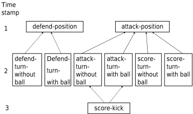
The hypotheses graph is a connected graph G′ , whose vertices correspond to successfully-tagged paths in the plan library (i.e., hypotheses). Edges in G′ connect hypothesis vertices tagged with time stamp t to hypothesis vertices tagged with time stamp t + 1. G′ is therefore constructed in levels, where each level represents hypotheses that hold at the corresponding time stamp. For each set of observations made at time ti, we add to G′ a level ti, with nodes for all current state hypotheses that were successfully tagged t = t0. We then create edges between vertices x1, . . . , xn in level ti to vertices y1, . . . , ym in level ti-1 in the following manner: If xi is not part of a sequence (i.e., it is a first child), then we connect xi to each vertex yj, (j = 1...m); otherwise, if xi is part of a sequence, we connect xi to yj if any of the plans in yj has a sequential edge to a plan in xi. Finally, if xi is equal to yj , we connect them to allow for the self-cycles.

To generate all sequences of plan paths that are consistent with the observations, we traverse G′ from the last level ti backwards, to level ti-1, and on to the first level. Paths that connect level ti to level t = 1 denote valid state histories. To illustrate, Figure 2 shows G′ for the example above, t = 3.

Complexity Analysis. Let L be the worst-case number of plans that match a single observation. For each node in G′ with time stamp t (of which there could be at most O(L)), we check all nodes in time stamp t-1 (again, O(L)), thus a factor of L2 for each additional level. Thus over N observations, the worst-case runtime is O(NL2 ).

5 Experiments

We show results of experiments evaluating these techniques with simulated plan libraries and observation sequences. We controlled key parameters, such as the library size L, and the number of features used by each single plan f (f ≤ 10), and the structure of temporal edges. In the experiments below, L was set by modifying the number of top-level plans (children of the root node), and the depth of the library. The branching factor was fixed at 3. The maximum length of observation sequence was 10.

We generated valid sequences of observations by simulating execution and selection of plan steps. The process randomly chose a path in the library and used all the features in this path to generate observations. Based on existence of sequential edges, the process chose to either continue execution along a sequential edge, or jump to a new first child. In all experiments, we contrasted the results with RESL [Kaminka and Tambe, 2000], the most relevant of the related works.

5.1 Matching Experiments

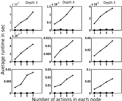
A first set of experiments compares matching run-time using FDT and RESL, as the plan library grows in size. We generated different-sized libraries by varying the library depth, and number of top-level plans. To demonstrate the scale-up offered by the FDT as the observation complexity grows, we also vary f (1,3,5,7). For each of these values, we generated 180 random observations sets based on the plan-libraries, and averaged the run-time for matching these using RESL and using an automatically constructed FDT.

The average matching runtime is shown in Figure 3. The figures are arranged in a 3 × 3 matrix. The rows correspond to the number of top-level plans (5, 50, and 100, respectively, top-down). The columns correspond to library depths of 3,4 and 5. Thus the bottom right figure shows the results for the largest library, approximately 12,101 nodes. The FDTs for these included 200-2000 nodes, depending on the number of features associated with each plan (f). In all figures, the horizontal (X) axis shows f, and the vertical axis shows the average matching time in seconds. Each point in a figure is the average of 180 runs.

Clearly, the use of the FDT leads to very significant improvements in the matching time, compared to RESL-and even when each plan is associated with a single atomic observation. Furthermore, its growth curve indicates that its benefits are maintained even as the observations increase in complexity.

5.2 Query Answering Algorithms

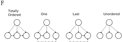
We now turn to evaluate the algorithms answering the currentstate and state-history queries. These answers depend critically on the temporal structure of the plan library, in terms of sequential edges. We follow [Geib and Harp, 2004] in varying temporal structure in several ways (Fig. 4): (a) Totally Number of actions in each node ordered: all children of same parent form a single chain; (b) First: first child has sequential edge to all its siblings; (c) Last: siblings have sequential edges leading to the last sibling; (d) Unordered: no ordering constraints between nodes. Top-level plans are always unordered.

Propagation Accuracy. A key advantage of CSQ over RESL is its ability to use sequential edges and the history of observations to rule out hypotheses that are temporally inconsistent (Section 4.1). Given a sequence of observations, we expect to see fewer current state hypotheses in comparison with RESL.

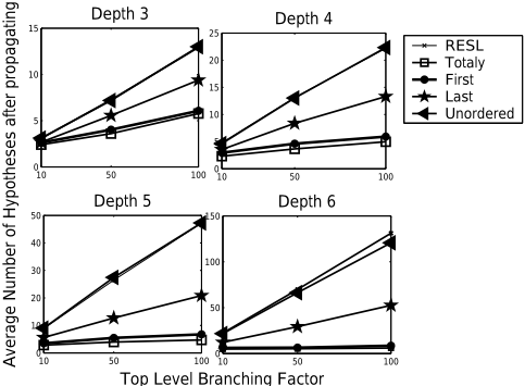
We again varied the library size through the number of toplevel plans (10,50,100) and the depth of the plan library (36). We vary the temporal structure of the library as described above. Trials were conducted with sequences of 10-40 observations. We recorded the number of hypotheses maintained after each observation was propagated.

Figure 5 shows the effect of sequential edges types on the number of hypotheses. There are four figures, each for different depth (3-6). The X axis shows the number of top-level plans, while the Y axis measures the average number of hypotheses across all trials of the same configuration. Each data point reflects the average number of hypotheses over 3000 individual observations, organized as 120 random observation sequences (each 10-40 observations in length), based on the generated libraries.

The figures show that totally-ordered libraries allow CSQ to maximally use past observations, and thus result in less hypotheses. In contrast, unordered libraries have no sequential edges, and thus do not gain information from a history of observations. Thus the number of hypotheses generated in this case is exactly the same as generated by RESL-which ignores such history in any case (and thus its results for all library types are the same, shown in a single solid line). On average, more than 50% of the current state hypotheses generated by RESL were ruled out by the CSQ propagation.

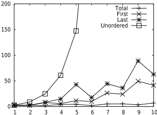
We also show the results of evaluating the state history algorithm. Figure 6 shows how incoming observations affect the number of state history hypotheses. The X axis shows the progression of 10 observations with time. The Y axis shows the number of state history hypotheses generated by traversing the hypotheses graph G′ . The totally ordered libraries have very few hypotheses, while the number of hypotheses for unordered libraries grows exponentially, since all combinations of current-state hypotheses are valid.

Propagation Runtime. Given the significant improvement in accuracy, one may expect an associated significant computational cost in CSQ, compared to RESL. We have argued analytically that this is not the case, and this is supported empirically. Figure 7 shows the average run-time of CSQ in the above experiments, in comparison to RESL's. The X axis shows the number of top-level plans, while the Y shows runtime in seconds. RESL is only slightly faster than CSQ. Indeed, the difference in propagating between CSQ and RESL amounts to a few additional checks (for incoming edges).

6 Summary and FutureWork

This paper presents methods for efficient, complete, symbolic plan recognition that can answer a variety of recognition queries, with increased accuracy. The algorithms depart from previous approaches in that they take a lazy-commitment ap- Top Level Branching Factor proach, separating the current state and state history queries, and implicit representation of hypotheses, until required. In addition, we presented a novel application of decision tree construction for efficiently matching observations to the plan library-a step common to all plan recognition methods. We plan to further explore the use of symbolic algorithms in additional queries.

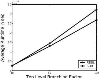
Figure 7: Average runtime of propagating RESL versus CSQ

Acknowledgments. This research was supported in part by the Israeli Ministry of Commerce, and by ISF grant #1211/04. Special thanks to Nadav Zilberbrand and K.Ushi.