
Breaking symmetries in all different problems
Proceedings of the Nineteenth International Joint Conference on Artificial Intelligence. Pages 272-276.
© 2005 International Joint Conferences on Artificial Intelligence
Abstract
Adding symmetry breaking constraints is one of the oldest ways of breaking variable symmetries for CSPs. For instance, it is well known that all the symmetries for the pigeon hole problem can be removed by ordering the variables. We have generalized this result to all CSPs where the variables are subject to an all different constraint. In such case it is possible to remove all variable symmetries with a partial ordering of the variables. We show how this partial ordering can be automatically computed using computational group theory (CGT). We further show that partial orders can be safely used together with the GE-tree method of [Roney-Dougal et al., 2004]. Experiments show the efficiency of our method.
- [Crawford et al., 1996] Crawford, J., Ginsberg, M., Luks E.M., Roy, A. "Symmetry Breaking Predicates for Search Problems." In proceedings of KR'96, 148-159.
- [Flener et al., 2002] P. Flener, A. M. Frisch, B. Hnich, Z. Kiziltan, I. Miguel, J. Pearson, T. Walsh.: "Breaking Row and Column Symmetries in Matrix Models. " Pro- ceedings of CP'02, pages 462-476, 2002 [
- [ILOG, 2003] ILOG: ILOG Solver 6.
- User Manual. ILOG, S.A., Gentilly, France, Septembre 2003 [
- [Lustig and Puget, 2001] Lustig, I.J., and Puget, J.F. (2001). "Program Does Not Equal Program: Constraint Pro- gramming and its Relationship to Mathematical Pro- gramming," Interfaces 31(6), 29-53.
- [Mc Kay, 1981] Mc Kay, B.: "Practical Graph Isomor- phism" Congr. Numer. 30, 45-87, 1981
- [Ollerenshaw, 1986] Dame Ollenrenshaw, K. "On most per- fect or complete 8x8 pandiagonal magic squares" Pro- ceedings Royal Society London, 407, 259-281, 1986.
- [Petrie and Smith, 2003] Petrie, K., Smith, B.M. : "Sym- metry breaking in graceful graphs." In proceedings of CP'03, LNCS 2833, 930-934, Springer Verlag, 2003.
- [Petrie, 2004] Petrie, K. : "Combining SBDS and SBDD" Technical report APES-86-2004. Available from http://www.dcs.st-and.ac.uk/˜apes/apesreports.html" Link
- [Puget, 1993] Puget, J.-F.: "On the Satisfiability of Symmet- rical Constraint Satisfaction Problems." Proceedings of ISMIS'93 (1993), 350-361.
- [Roney-Dougal et al., 2004] Roney-Dougal C.M., Gent, I.P., Kelsey T., Linton S.: "Tractable symmetry breaking us- ing restricted search trees" To appear in proceedings of ECAI'04.
- [Roy and Luks, 2004] Roy. A., Luks, E.: "The complexity of symmetry-breaking formulas", Annals of Mathematics and Artificial Intelligence , 41 (2004), 19-45 (with A. Roy).
- [Seress, 2003] Seress, A.: Permutation Group Algorithms Cambrige University Press, 2003.
References were extracted automatically from the PDF and may contain errors.
Full text extracted automatically from the PDF; figures, tables and equations may differ. The PDF is the version of record.
1 Introduction
A symmetry for a Constraint Satisfaction Problem (CSP) is a mapping of the CSP onto itself that preserves its structure as well as its solutions. If a CSP has some symmetries, it may be the case that all symmetrical variants of every dead end encountered during the search must be explored before a solution can be found. Even if the problem is easy to solve, all symmetrical variants of a solution are also solutions, and listing all of them may just be impossible in practice. Those observations have triggered a lot of interest for the detection and removal of symmetries in the constraint programming community. Adding symmetry breaking constraints is one of the oldest ways of breaking variable symmetries for (CSPs). For instance, it is shown in [Crawford et al., 1996] that all variable symmetries could be broken by adding one lexicographical ordering constraint per symmetry. Unfortunately, this method is not tractable in general, as there may be an exponential number of symmetries. It has been shown that in general there is no way to break all symmetries of a problem with a polynomial number of constraints[Roy and Luks, 2004]. In [Flener et al., 2002], a linear number of constraints are used to break symmetries for matrix problems. As expected, since there are a polynomial number of constraints, not all symmetries are broken. However, a polynomial number of constraints may be sufficient for breaking all symmetries in some special cases. For instance, in [Puget, 1993], it is shown that a linear number of constraints can break all symmetries for the pigeon hole problem: one simply needs to order the variables. In this paper we consider a more general class of problems: all different problems. These are CSPs such that the variables are subject to an all different constraint among other constraints. We show in section 4 that for such CSPs, all variable symmetries can be broken with at most n - 1 binary constraints, where n is the number of variables.
In [Roney-Dougal et al., 2004] a general purpose method for breaking all value symmetries is given: the GE-tree method. We show in section 5 that this method can be safely combined with symmetry breaking constraints, under some conditions on the order in which the search tree is traversed.
In section 6, we apply our method to some complex CSPs. We summarize our findings and discuss some possible generalizations in section 7.
2 Symmetries, Graphs and CSPs
The symmetries we consider are permutations, i.e. one to one mappings (bijections) from a finite set onto itself. Without loss of generality, we can consider permutations of I n , where I n is the set of integers ranging from 0 to n - 1. For instance, we can label the variables of a graph with integers, such that any variable symmetry is completely described by a permutation of the labels of its variables. This is formalized as follows.
2.1 Computational Group Theory
Let Sn be the set of all permutations of the set I n . The image of i by the permutation σ is denoted iσ . A permutation σ ∈ Sn is fully described by the vector [0σ , 1σ , . . . , (n-1)σ ]. The product of two permutations σ and θ is defined by i(σθ) = (iσ )θ .
Given i ∈ I n and a permutation group G ⊆ Sn , the orbit of i in G, denoted iG, is the set of elements to which i can be mapped to by an element of G:
Given i ∈ I n and a permutation group G ⊆ Sn , the stabilizer of i in G, denoted iG, is the set of permutations of G that leave i unchanged:
2.2 CSP and symmetries
A constraint satisfaction problem P (CSP) with n variables is a triple P = (V,D, C) where V is a finite set of variables (vi)i∈I n, D a finite set of finite sets (Di)i∈I n, and every constraint in C is a subset of the cross product ⊗i∈I n Di. Without loss of generality, we can assume that Di ⊆ I k for some k.
An assignment is a member of S, i.e. a vector of values (ai)i∈I n such that ai ∈ Di for all i ∈ I n , and is denoted (vi = ai)i∈I n. A partial assignment is sub vector of an assignment.
A solution to (V,D, C) is an assignment that is consistent with every member of C.
Given a permutation σ of I n , we define a variable permutation on (partial) assignments as follows:
Such permutation is called a variable symmetry if it maps solutions to solutions.
Given a permutation θ of I k , we define a value permutation on (partial) assignments as follow:
Such permutation is called a value symmetry if it maps solutions to solutions.
2.3 A graph coloring example
Let us introduce an example that will be used throughout the paper. We say that a graph with m edges is graceful if there exists a labeling f of its vertices such that:
- 0 ≤ f(i) ≤ m for each vertex i,
- the set of values f(i) are all different,
- the set of values abs(f(i), f(j)) for every edge (i, j) are all different.
A straightforward translation into a CSP exists where there is a variable vi for each vertex vi, see [Lustig and Puget, 2001]. The variable symmetries of the problem are induced by the automorphism of the graph. There is one value symmetry, which maps v to m - v. More information on symmetries in graceful graphs is available in [Petrie and Smith, 2003], [Petrie, 2004].
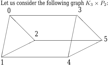
The group of variable symmetries of the corresponding CSP is equivalent to the group of symmetries of the graph. Such group can be computed by packages such as Nauty[Mc Kay, 1981]. This group G is:
3 Breaking variable symmetries
Without loss of generality, we can assume that domains are subsets of I k for some k, with the usual ordering on integers.
3.1 Lex leader constraints
Adding constraints is one of the oldest methods for reducing the number of variable symmetries of a CSP[Puget, 1993]. In [Crawford et al., 1996], it is shown that all the variable symmetries of any CSP can be broken by the following constraints.
For a given σ, the constraint (V ⪯ V σ ) is semantically equivalent to the disjunction of the constraints:
If the last constraint is omitted, the set of constraints is denoted V ≺ V σ .
In our example, the constraints given by [Crawford et al., 1996] are
3.2 A polynomial number of constraints
The number of constraints (1) can grow exponentially with the number of variables V. Using the fact that the variable are subject to an all different constraint, we can significantly reduce the number of symmetry breaking constraints. Let us consider one of the symmetries of our example, namely:
The constraint breaking this symmetry is
Since v0 = v0 is trivially true, and since v1 = v2 cannot be true because of the all different constraint, this constraint can be simplified into:
This simplification is true in general and can be formalized as follows. Given a permutation σ, let s(σ) be the smallest i such that iσ ̸= i, and let t(σ) be equal to (s(σ))σ .
Lemma 1. Given a CSP where the variables V are subject to an all different constraint, and a variable symmetry group G for this CSP, then all variable symmetries can be broken by adding the following constraints:
Proof. By definition kσ = k for all k < s(σ), and s(σ)σ ̸= s(σ). Let us look at the constraint V ⪯ Vσ. There is an all different constraint on the variables V, which means that vi = viσ if and only if iσ = i. In particular, vk = vkσ for all k < s(σ), and vs(σ) ̸= v(s(σ))σ . Therefore, only one disjunct for the constraint can be true, namely:
Since kσ = k for k < s(σ) and s(σ)σ = t(σ), this can be simplified into vs(σ) < vt(σ). ✷
Note that if two permutations σ and θ are such that s(σ) = s(θ) and t(σ) = t(θ), then the corresponding symmetry breaking constraints are identical. Therefore, it is sufficient to state only one symmetry breaking constraints for each pair i, j such that there exists a permutation σ with i = s(σ) and j = t(σ).
The set of these pairs can be computed using what is known as the Schreier Sims algorithm [Seress, 2003]. This algorithm constructs a stabilizers chain G0, G1, . . . , Gn as follows:
By definition,
The Schreier Sims algorithm also computes set of coset representatives Ui. Those are orbits of i in Gi:
By definition, Ui is the set of values which i is mapped to by all symmetries in G that leave at least 0, . . . , (i - 1) unchanged.
From now on, we will assume that all the groups we use are described by a stabilizers chain and coset representatives. In our example, the stabilizer chain is :
All remaining stabilizers G3,G4,G5 are equal to G2. Coset representatives are:
Theorem 2. Given a CSP with n variables V such that there exists an all different constraint on these variables, and given coset representatives sets Ui for the variable symmetry group of the CSP, then all the variable symmetries can be broken by at most n(n - 1)/2 binary constraints. These constraints are given by :
Proof. By definition, for each element j ∈ Ui, there exists at least one permutation σ ∈ Gi such that iσ = j and j = t(σ). The converse is also true. If there exists a permutation σ such that i = s(σ) and that j = t(σ), then j ∈ Ui. Therefore, the constraints (2) can be rewritten into:
There are ∑n-1 i=0 (|Ui| - 1) such constraints. All the permutations of Gi leave the numbers 0, . . . , i - 1 unchanged. Therefore Ui is a subset of {i, . . . , n - 1}. Then |Ui| - 1 ≤ n - i - 1. Therefore, the number of constraints is bounded from above by ∑n-1 i=0 (n - i - 1) = n(n - 1)/2. ✷
In our example, these constraints are :
Note that some of these constraints are redundant. For instance, the constraint v0 < v2 is entailed by the first and the last constraints. This remark can be used to reduce the number of constraints as explained in the following section.
3.3 A linear number of constraints
The previous result can be improved by taking into account the transitivity of the < constraints. Given j ∈ I n , it may be the case that j belongs to several of the sets Ui. In such case, let us define r(j) as the largest i different from j such that j belongs to Ui. If j belongs to no Ui other than Uj, then let r(j) = j.
Before stating our main result, let us prove the following.
Lemma 3. With the above notations, if j ∈ Ui and i ̸= j then r(j) ∈ Ui and r(j) < j
Proof. Let us assume that j ∈ Ui and i ̸= j. By definition of Ui there exists a permutation σ ∈ Gi such that iσ = j. Let k = r(j). By definition of r(j), i ≤ k and j ∈ Uk. Therefore, there exists a permutation θ ∈ Gk such that kθ = j. Let ν = σθ-1 . Then, iν = iσθ-1 = j θ-1 = k. Moreover, ν ∈ Gi because σ ∈ Gi and θ ∈ Gk ⊆ Gi. Therefore, k ∈ Ui. The fact that r(j) < j is an immediate consequence of the definition of r(j).✷
We can now state our main result.
Theorem 4. With the above notations, given a CSP with n variables V, such that there exists an all different constraint on these variables, then all variable symmetries can be broken by at most n - 1 binary constraints. These constraints are given by :
Proof. The number of constraints (4) is at most n by definition. Note that r(0) = 0 by definition of r, therefore, the number of constraints is at most n-1. Let us consider one of the constraints of (3). We are given i and j such that j ∈ Ui and i ̸= j. We want to prove that the constraint c = (vi < vj) is implied by the constraints (4). Let us consider the sequence (j, r(j), r(r(j)), r(r(r(j))), . . .). Let us assume that the sequence never meets i. We have that j ∈ Ui and i ̸= j. By application of lemma 3, we get r(j) ∈ Ui and r(j) < j. Since r(j) ̸= i by hypothesis, lemma 3 can be applied again. By repeated applications of lemma 3 we construct an infinite decreasing sequence of integers all included in Ui. This is not possible as Ui is finite. Therefore, there exists k such that i = rk (j). Moreover, we have established rk (j) ̸= rk-1 (j), . . . , r(r(j)) ̸= r(j), r(j) ̸= j. Therefore, the constraints vrk (j) < vrk-1 (j), . . . vr(r(j)) < vr(j), vr(j) < vj are constraints of (4). Together they imply vrk (j) < vj which is the constraint c. We have proved that the constraints (3) are implied by the constraints (4). Since the set of constraints (4) is a subset of the constraints (3), both sets of constraints are equivalent. Then, by theorem 2, the constraints (4) break all variable symmetries. ✷
In our example, we get from coset representatives:
Therefore, the constraints (4) given by theorem 4 are:
Note that the constraint v0 < v2 is no longer appearing.
4 Breaking both variable symmetries and value symmetries
In [Roney-Dougal et al., 2004], a general method for breaking all value symmetries is described. This method uses the group of value symmetries of the CSP. We will show that this method can be combined with symmetry breaking constraints when there are both variable symmetries and value symmetries.
4.1 GE-tree and symmetry breaking constraints
We are given a CSP P with n variables vi subject to an all different constraint among other constraints. Without loss of generality, we can assume that the domains of the variables are subsets of I k for some k. It is shown in [Flener et al.,
2002] how to transform P into a new CSP P ′ such that all value symmetries of P become variable symmetries of P ′ . The idea is to add n×k additional binary variables xij (variables with domains equal to {0, 1}). We also add the following channeling constraints:
These constraints state that the variable xij equals 1 if and only if the variable vj equals j. Adding these new variables do not change the solutions of the CSP. Moreover, variable symmetries of P are equivalent to permutations of the rows of the xij matrix, whereas value symmetries of P are equivalent to permutations of the columns of the same matrix.
Let us construct the vector X by concatenating the rows of the matrix xij. Therefore, the variables xij are ranked in increasing values of i then increasing values of j in the vector X.
Let us consider a value symmetry θ for P. Then θ is a permutation of the matrix columns. This symmetry is broken by the constraint:
Let Xi be the variables in the i-th row of the matrix. The value symmetry θ maps variables in a given row to variables in the same row. This is formalized as follows.
From the definition of ⪯, we have that (5) is equivalent to the disjunction of the following constraints:
Let us compare lexicographically Xi with (Xθ )i. Let ai be the value assigned to vi. Then xi(ai) = 1 and xij = 0 for j ̸= ai. Similarly, xi(j)θ-1 = 1 if and only if j θ-1 = ai, i.e. aθi = j. Therefore, Xi = (Xθ )i if and only if ai = (ai)θ , and Xi ≺ (Xθ )i if and only if ai < (ai)θ .
We then have that (5) is equivalent to the disjunction of the constraints:
Let us now consider one of the disjunct, namely:
This means that θ leaves invariant a0, a1, . . . , ai-1. In such case ai must be minimal among the values that any such θ can map it to. We have therefore proved the following result.
Lemma 5. With the above notations, ai is the minimum of its orbit in the group of symmetries that leave a0, a1, . . . ai-1 unchanged.
This is equivalent to the GE-tree method for breaking all value symmetries [Roney-Dougal et al., 2004], when the variables and the values are tried in an increasing order during search.
From [Crawford et al., 1996], it is safe to add all possible symmetry breaking constraints (1) on P ′ . In particular, it is safe to state all the constraints (1) for the variable symmetries of P together with all the constraints (5). By lemma 5, the set of constraints (5) is equivalent to the GE-tree method for breaking value symmetries. We have just proved the following result.
Theorem 6. Given a CSP, its group of variable symmetries G1, and its group of value symmetries G2, then the combination of the GE-tree method for breaking value symmetries with the symmetry breaking constraints (1) computes a set of solutions S such that:
Theorem 4 in section 3 says that the set of all those constraints (1) is equivalent to the constraints (4) when there is an all different constraints on all the variables V. This yields the following result.
Corollary 7. Given a CSP where the variable are subject to an all different constraint, its group of variable symmetries G1, and its group of value symmetries G2, then the combination of the GE-tree method for breaking value symmetries with the symmetry breaking constraints (4) computes a set of solutions S such that:
5 Experimental results
We have implemented an algorithm similar to Nauty[Mc Kay, 1981] for computing graph automorphisms, as well as a Schreier Sims algorithm[Seress, 2003]. These have been used in the following examples. In our implementation, we did not fully implement the GE-tree method, because it requires more computational group algorithms than what we have implemented so far. We simply compute the orbits for the group G of value symmetries. Then, only the minimum element of each orbit is left in the domain of the variable v0. We will refer to this method as SBC (for Symmetry Breaking Constraints) in order to differentiate it from other methods.
5.1 Graceful graphs
We have tested our approach on the graceful graphs of [Petrie and Smith, 2003]. Variable symmetries are broken by the constraints (4). There is one non trivial value symmetry, which maps a to e - a; where e is the number of edges of the graph. Therefore, the orbits for this symmetry are the sets {a, e - a}, for 0 ≤ a ≤ e/2. Therefore, one can restrict the domain of v0 by keeping one the smallest value in each of these orbits.
For each graph we report the number of solutions of the CSP (sol), the size of the search tree (node) and the time (time) needed to compute all these solutions the running time without symmetry breaking technique (no sym). We also report these figures when the SBC method is used. In this case the running time includes the time needed to perform all the group computations. Running times are measured on a 1.4 GHz Dell Latitude D800 laptop running Windows XP. The implementation is done with ILOG Solver 6.0[ILOG, 2003].
| graph | no sym | SBC | ||||
|---|---|---|---|---|---|---|
| sol | node | time | sol | node | time | |
| K3 × P2 | 96 | 1518 | 0.12 | 8 | 83 | 0.01 |
| K4 ×P2 | 1440 | 216781 | 13.6 | 30 | 1863 | 0.27 |
| K5 ×P2 | 480 | 34931511 | 4454 | 2 | 53266 | 6.5 |
| K6 × P2 | 0 | 1326585 | 305 | |||
The running times are up to 30 times smaller than the ones reported in [Petrie, 2004] for the GAP-SBDD and the GAPSBDS methods, using a computer about half the speed of ours. This shows that in this example our symmetry breaking constraints are much more efficient than modified search methods. However, we find twice as many more solutions. Let see why on the graph K5 × P2. This graph has 10 vertices and 25 edges. We list the values for the variables v0, v1, . . . , v9 for the two solutions:
Let us apply the non trivial value symmetry to the second one. We get:
Let us apply the following variable symmetry to it:
This yields the first solution!
This example shows that we did not break all symmetries that are a product of a variable symmetry by a value symmetry. This is so despite the fact that all variable symmetries and all value symmetries are broken.
5.2 Most Perfect Magic Squares
Most perfect magic squares, studied in [Ollerenshaw, 1986], are given as an example of a CSP with convoluted variables symmetries in [Roney-Dougal et al., 2004]. The authors decided to use an inverse representation in order to transform variable symmetries into value symmetries. These were in turn broken with the GE-tree method. In [Ollerenshaw, 1986], it is proven that most perfect magic squares are in a one to one relationship with reversible squares. A reversible square of size n×n (where n ≡ 0 mod 4) has entries 1 . . . n2 such that (i) the sum or the two entries at diagonally opposite corners of any rectangle or sub-square equals the sum of the other pair of diagonally opposite corners (ii) in each row or column, the sum of the first and last entries equals the sum of the next and the next to last number, etc (iii) diametrically opposed numbers sum to n2 + 1.
Any solution is one of 2n+1 ((n/2)!)2 symmetric equivalent[Ollerenshaw, 1986]. For n = 16, this is about 2.13e+14.
The natural model for this problem has one variable per cell in the square with entries as values. In addition to the above constraints on entries, there is an all different constraint. Therefore, our variable symmetry breaking constraints can be used. We report for various sizes the time used to compute the symmetry breaking constraints as well as the time for finding all non symmetrical solutions with our SBC method. We also report the results of [Roney-Dougal et al., 2004], obtained with GAP-SBDD and with GE-tree on a computer about half the speed of ours. A direct comparison is difficult because they directly search for most perfect magic squares whereas we search for reversible squares. It is worth comparing the time spent in the symmetry computations though, because these deal with the same symmetry group. Our method spends much less time in symmetry computations because this needs to be done only once, before the search starts.
| Method | n | sols | sym | search |
|---|---|---|---|---|
| SBC | 4 8 12 | 3 10 42 | 0.01 0.09 0.44 | 0.02 0.39 22.2 |
| 16 4 8 | 35 3 | 4.6 0.3 | 275.6 0.3 125.4 | |
| GAP-SBDD | 10 | 5.4 | ||
| GE-tree | 12 | 42 | 2745 0.2 | |
| 4 8 | 3 10 | 0.7 | 0.1 90.0 | |
| 12518 | ||||
| 12 | 42 | 29.1 | 10901.8 |
6 Discussion
We have established two major results (i) all variable symmetries can be broken by a linear number of binary constraints if there is an all different constraints on all the variables of the CSP (ii) symmetry breaking constraints of [Crawford et al., 1996] can be safely used in conjunction with the GE-tree method of [Roney-Dougal et al., 2004].
Furthermore, these methods can be fully automated using automorphism packages such as Nauty[Mc Kay, 1981] and computational group theory[Seress, 2003]. We have implemented such algorithms. Experiments on complex problems show that these algorithms are quite efficient.
The results described in this paper can be generalized. First of all, theorem 4 is valid for all CSPs where the variables are subject to an all different constraint. It would be interesting to see if similar results can be obtained for other forms of CSPs.
It is worth mentioning that we presented a method for breaking all variable symmetries, and all value symmetries. However, our method does not break products of both kinds of symmetries. It remains to be seen if a simple combination of variable and value symmetry breaking techniques can break all such symmetries.
Acknowledgements
The author would like to thank Marie Puget and the anonymous referees for their remarks. It greatly helped improving the readability of this paper.
@inproceedings{ijcai2005p150,
  title     = {Breaking symmetries in all different problems},
  author    = {Puget, Jean-Francois},
  booktitle = {Proceedings of the Nineteenth International Joint Conference on
               Artificial Intelligence, {IJCAI-05}},
  publisher = {International Joint Conferences on Artificial Intelligence},
  editor    = {Leslie Pack Kaelbling and Alessandro Saffiotti},
  pages     = {272--276},
  year      = {2005},
  url       = {https://ijcai.org/proceedings/2005/150},
}
TY - CPAPER TI - Breaking symmetries in all different problems AU - Puget, Jean-Francois T2 - Proceedings of the Nineteenth International Joint Conference on Artificial Intelligence, IJCAI-05 PB - International Joint Conferences on Artificial Intelligence PY - 2005 SP - 272 EP - 276 UR - https://ijcai.org/proceedings/2005/150 ER -Copied
Machine-readable versions of this paper, for tools and AI agents:





