
Skewing: An Efficient Alternative to Lookahead for Decision Tree Induction
Proceedings of the Eighteenth International Joint Conference on Artificial Intelligence. Pages 601-611.
© 2003 International Joint Conferences on Artificial Intelligence
Abstract
This paper presents a novel, promising approach that allows greedy decision tree induction algorithms to handle problematic functions such as parity functions. Lookahead is the standard approach to addressing difficult functions for greedy decision tree learners. Nevertheless, this approach is limited to very small problematic functions or subfunctions (2 or 3 variables), because the time complexity grows more than exponentially with the depth of lookahead. In contrast, the approach presented in this paper carries only a constant run-time penalty. Experiments indicate that the approach is effective with only modest amounts of data for problematic functions or subfunctions of up to six or seven variables, where the examples themselves may contain numerous other (irrelevant) variables as well.
- [Blake and Merz, 1998] C.L. Blake and C.J. Merz. UCI repository of machine learning databases, 1998.
- [Breiman eta/., 1984] L. Breiman, J.H. Friedman, R.A. Olshen, and C.J. Stone. Classification and Regression Trees. Wadsworth and Brooks/Cole, Monterey, 1984.
- [Breiman, 1996] L. Breiman. Bagging predictors. Machine Learn- ing, 24(2):123-140, 1996.
- [Elidan eta/., 2002] G. Elidan, M. Ninio, N. Friedman, and D. Schuurrnans. Data perturbation for escaping local maxima in learning. In AAAI-02/IAAI-02, pages 132-139, 2002.
- [Freund and Schapire, 1997] Y. Freund and R. Schapire. A decision-theoretic generalization of on-line learning and an ap- plication to boosting. Journal of Computer and System Sciences, 55:119-139, 1997.
- [Friedman et al., 1999] Nir Friedman, Iftach Nachman, and Dana Peer. Learning bayesian network structure from massive datasets : The "sparse candidate" algorithm. In UAI-99, pages 206-215, 1999.
- [Norton, 1989] S. Norton. Generating better decision trees. In /JCA/-89, pages 800-805, 1989. IJCAI
- [Quinlan, 1983] J.R. Quinlan. Learning efficient classification pro- cedures and their application to chess end games. In R.S. Michal- ski, J.G. Carbonell, and T.M. Mitchell, editors, Machine Learn- ing I, chapter 15, pages 463-482.
- [Quinlan, 1997] J.R. Quinlan. C4.5: Programs for Machine Learn- ing. Kaufmann, 1997.
- [Szallasi, 2001] Z. Szallasi. Genetic network analysis : From the bench to computers and back. In Tutorial Notes, Second International Conference on Systems Biology, 2001. www.icsb200 1.org/SzallasiTutorial. pdf. Link
References were extracted automatically from the PDF and may contain errors.
Full text extracted automatically from the PDF; figures, tables and equations may differ. The PDF is the version of record.
1 Introduction
Algorithms for the top-down induction of decision trees (TDIDT) are among the most widely used algorithms for machine learning, data mining and statistical classifica tion. TDIDT implementations such as ID3 [Quinlan, 1983], C4.5 [Quinlan, 1997], C5.0 (www.rulequest.com) and CART [Breiman eta/., 1984] are easy to use and (often) produce human-comprehensible models. Nevertheless, TDIDT algo rithms are well-known to be myopic because of their greedy strategy for choosing split variables, or internal node labels. This myopia is at its worst when the data are labeled accord ing to parity functions such as exclusive-or (2-bit odd parity, denoted by EB ). These and related other problematic functions naturally arise in real-world data. For example, in fruitfly ex periments, flies that are either male and have an active Sxl gene or that are female and have an inactive Sxl gene survive, while other flies die; hence survival is an exclusive-or func tion of gender and Sxl activity (Table 1).
Of course, parity and parity-like functions are also prob lematic for other machine learning or statistical algorithms that employ (explicitly or implicitly) a linear assumption in order to gain efficiency. Such models include perceptrons, logistic regression, linear support vector machines, Fischer's linear discriminant and naive Bayes. They also include any of Soumya Ray t· sray@cs.wisc.edu t Department of Computer Sciences University of Wisconsin Madison, Wisconsin 53706
| Gender Female | Sxl active | Survival |
|---|---|---|
| 0 0 1 1 | 0 1 0 1 | 0 1 1 0 |
a variety of data analysis approaches that employ an informa tion gain or Kullback-Leibler divergence filter to do variable selection or to control computation time, for example as in the sparse candidate algorithm for learning Bayesian networks [Friedman eta/., 1999]. The inability of such approaches to learn functions like EB is frequently noted, for example, in the context of analyzing gene expression microarray data [Fried man eta/., 1999; Szallasi, 200 1].
In TDIDT algorithms, the myopia of the search can be re duced at the cost of increased computation time. The stan dard approach is through depth-k lookahead [Norton, 1989], where the default for TDIDT algorithms is depth-1 looka head. However, the time to perform a split grows exponen tially with k, and problematic functions remain no matter how large a k is chosen.
The purpose of this paper is to introduce an alternative ap proach to problematic functions such as parity, which does not incur the high computational cost of lookahead. The ap proach relies on the observation that these functions are not actually problematic if the distribution over the data is signif icantly different from uniform. In such cases other functions may become problematic for TDIDT algorithms, but func tions such as exclusive-or become relatively easy. Hence we first observe that TDIDT algorithm performance on a data set can be improved if the algorithm has access to a second, sig nificantly different distribution over the data. Of course such a second distribution often is unavailable. Therefore, we next show how the second distribution often can be simulated by skewing the data from the first distribution. We note that the present paper focuses entirely on classification, ignoring re gression trees, or trees that predict continuous outputs at their leaves. Furthermore, we limit our entire discussion to TDIDT algorithms that perform only binary splits, although the data may use variables that can take more than two values.
| X1 | Xz | X3 f |
| 0 | 0 | 0 1 |
| 1 | 0 | 1 0 |
| 0 | 1 | 0 0 |
| 0 | 1 | 1 1 |
2 Review of Lookahead for Hard Functions
We assume the reader is familiar with the approach ofTDIDT algorithms. The assumed familiarity includes a knowledge of the commonly-used functions to measure node purity, such as entropy [Quinlan, 1997] or Gini index [Breiman et al., 1984]. It also includes familiarity with the greedy heuristic of choos ing to split on the variable that maximizes the improvement, or gain, in the node purity score. We now review the notions of problematic functions and lookahead. For ease of discus sion, this section limits itself to two-class problems, where the classes are positive and negative.
For the various node purity functions employed by differ ent TDIDT algorithms, splitting on a variable Xi can yield a non-zero gain only if the class distribution changes for at least one of the values (or ranges) that Xi can take. If the distribution of classes is the same for every value of Xi (or range) then Xi will have zero gain according to any node pu rity measure in common usage. As an example, in Table 2 the variable x1 has non-zero gain according to either Gini or entropy, whereas the variables x2 and x3 have zero gain.
Consider a data set drawn from a uniform distribution over binary-valued variables x1 , x2 · · · x100 , labeled according to the target function Xgg EB x100 . Even if we are fortunate enough to have a complete data set-one occurrence of each truth assignment over x1 · · · x100-it is clear that for every variable Xi , the class distribution is exactly the same whether Xi is 0 or 1. So, regardless of how large a uniform sample we choose to draw, a variable will have non-zero gain only because of chance. Thus, the probability that one of the cor rect variables (xgg or x100) will have a higher gain than every one of the incorrect variables is extremely low. Hence the learning task is virtually impossible for a TDIDT algorithm.
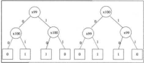
With depth-2 lookahead the preceding task becomes triv ial. A depth-2lookahead from a given node chooses not only the next split variable, but also the split variables at the next level. A TDIDT algorithm augmented in this way will con sider among the possible depth-2 trees the two shown in Fig ure 1, each of which will have the maximum possible gain. For any reasonably large data set, with high probability all other depth-2 trees will have gain only marginally different from zero. Hence we see that with depth-2lookahead, EB be comes easy. Because depth-2 lookahead is repeated at every step in tree construction, many other functions that have 2variable EB as a subfunction become easy.
Of course, depth-2lookahead comes with a price. Where n is the number of variables and m is the number of examples, the time to choose the split goes from O(mn) to O(mn 3 ), because labels have to be selected for three nodes from among n variables. Furthermore, there are many functions that require a higher lookahead. For example, suppose we have examples constructed from variables x1 · · · x 100 and the target is one of the functions in Table 3 involving x1 , x2 , and x 3 · Even with depth-2 lookahead, TDIDT is highly likely to choose incor rect variables. These problems can be solved with depth-3 lookahead, but the time to choose a split becomes O(mn 7 ), and other problematic targets remain even then. 1
| X1 | xz | X 3 | h | fz | h | !4 | h | !6 |
| 0 | 0 | 0 | 0 | 0 | 0 | 0 | l | 0 |
| 0 | 0 | 1 | 1 | 1 | 1 | 0 | 0 | 0 |
| 0 | 1 | 0 | 1 | 0 | 1 | 1 | 0 | 0 |
| 0 | 1 | 1 | 0 | 0 | 0 | 0 | 0 | 1 |
| 1 | 0 | 0 | 0 | 0 | 1 | 0 | 0 | 1 |
| 1 | 0 | 1 | 1 | 0 | 0 | 1 | 0 | 0 |
| 1 | 1 | 0 | 1 | 1 | 0 | 0 | 0 | 0 |
| 1 | 1 | 1 | 0 | 0 | 1 | 0 | 1 | 0 |
3 Motivation for Skewing
Consider the first target function discussed in the previous section, x 99 EB x 100 , but now suppose the data are distributed differently from uniform. For example, we might introduce dependencies not present in the uniform distribution: for ev ery odd number i, 1 :::; i :::; 99, if Xi is 0 then Xi+l has proba bility 0.99 of being 1. Or we might suppose all variables are independent as in the uniform distribution, but every variable has probability only t of taking the value 0. In either case, with a large enough sample we expect that the class distribu tion among examples with x99 = 0 will differ significantly from the class distribution among examples with x99 = 1.
To examine the preceding claim more closely, consider the second distribution, where each variable has probability t of being 0. If we draw a sample of 400 examples, we expect roughly 100 of these to have x99 = 0 and roughly 300 to have x9g = 1. Of the 100 with x99 = 0, we expect roughly ~ of these, or 75, to have x 100 = 1 and hence to belong to the positive class. Of the 300 with x99 = 1, we expect only t of these, or 75 again, to belong to the positive class (to have x10o = 0). Hence the fraction of positive examples is quite different for the two values of x99 : ~ of the examples with Xgg = 0 are positive, while t of the examples with x99 = 1 are positive. As a result x99 (and x100 ) will have non-zero gain; for instance, information gain is roughly 0.19 (out of maximum 1.0 possible) and Gini gain is roughly 0.06 (out of maximum 0.25 possible). On the other hand, every vari able other than x99 or x100 is likely to have nearly zero gain. Hence unless a highly unlikely sample is drawn, a TDIDT al gorithm will choose to split on either x99 or x100 , at which point the remainder of the learning task is trivial.
1 We can reduce this super-exponential growth of lookahead to "mere" exponential growth and still address parity-like functions if we require the tree to be "leveled"-all nodes at a level are labeled by the same variable. But even this non-standard lookahead proce dure imposes a high computational burden.
Notice that in the preceding discussion, moving to our sec ond distribution changed the marginal distribution for every variable, not just for those in the target. It would have re vealed the correct variables if the target function had been x2 EB X59 or even one of the problematic functions of three variables in Table 3. Notice also that the important aspect of the second distribution was that it changed the frequency distributions for the variables; the specific change for any variable could have gone the other way-to probability 2 of taking value 0-and the second distribution still would ~ave given non-zero gain to exactly the variables in the target.
From the preceding discussion we conclude that if we have access to two distributions that are "different enough," then choosing good variables to split on becomes relatively easy. However, in real-world problems we rarely have access to two different distributions over the data, or the ability to request data according to a second distribution that we choose. In stead, the next section discusses how in practice we can simu late a second distribution different from the first. We call this procedure skewing. The simulation approach tends to mag nify idiosyncrasies in the data set, for example, introducing some dependencies that were not present in the original dis tribution. Nevertheless, our experiments indicate that, if the data set is large enough, the magnification of idiosyncrasies is not a major problem.
4 Skewing Algorithm
The desired effect of the skewing procedure is that the skewed data set should exhibit significantly different frequencies from the original data set. Because we cannot draw new ex amples, we change the frequency distributions for variables by attaching various weights to the existing examples. The procedure initializes the weight of every example to 1. We next present · the details of the re-weighting procedure for binary-valued variables only. Nominal variables can be con verted to binary variables. We discuss extensions to continu ous variables in Section 7.
We may assume that every variable takes the value 0 in at least one example and takes the value 1 in at least one example-otherwise, the variable carries no information and can be removed. For each variable Xi, 1 < i < n, we ran domly, uniformly (independently for each -variable) select a "favored setting" Vi of either 0 or 1. We then increase the weight of each example in which Xi takes the value vi, by multiplying the weight by a constant; for the sake of illustra tion, suppose we double the weight.
At the end of this process, each example has a weight be tween 1 and 2n. It is likely that each variable has a signif icantly different weighted frequency distribution than previ ously, as desired. But this is not guaranteed. For example, suppose the original data set consists of 100 truth assignments over variables x1 and x2 . Suppose further that in half of these examples x1 = 0 and x2 = 1, and in the other half x1 = 1 and x2 = 0. If the favored setting for each variable happens to be 1, then all examples get assigned weight 2, so the new frequency distribution for each variable is the same as the original frequency distribution. In addition to this potential difficulty, a second difficulty is that this process can magnify idiosyncrasies in the original data. For instance, suppose we have a data set over x1 , ... , Xn, and (for simplicity) the favored setting for each variable is 1. If we happen to have one ex ample with many variables set to 1, it will get an inordinately high weight compared with other examples, potentially giv ing some insignificant variable a high gain. Can we mitigate these potential problems with the skewing procedure?
The difficulties in the preceding paragraph occur with some data sets combined with some choices of favored settings. Other selections of favored settings for the same data set may leave other variables' frequencies unchanged, but it is rela tively unlikely they will leave the same variables' frequencies unchanged. Furthermore, while other selections of favored settings may magnify other idiosyncrasies in the data, it is unlikely they will magnify the same idiosyncrasies. There fore, instead of using skewing to create only a second dis tribution, we use it to create some number T of additional distributions. The T different distributions come about from randomly (without replacement) selecting T different combi nations of favored settings for the n variables according to a uniform distribution. To ensure that tree construction is not thrown off course by any single bad distribution (either orig inal or skewed), the tree construction process is modified as described in the following paragraph.
Suppose we have T + 1 weightings of the data (the origi nal data set plus T reweighted versions of this data set), and we are considering a split. We score each of the n variables against each of the T + 1 weightings of the data. A variable that is not part of the target function should have nearly zero gain on every weighting, although as already noted, it may occur that on some weightings some of these variables can achieve high gain. But only variables that appear in the tar get should have significantly non-zero gain on most of the weightings (though not necessarily on all). Therefore, we set a gain threshold, and the variable that exceeds the gain threshold for the greatest number of weightings is selected as the split variable. Our expectation is that the selected variable is highly likely to be correct in the sense that it actually is a part of the target function. Yet the time for choosing the split remains O(mn), in contrast to lookahead. We have increased the run-time only by a small constant.
Pseudocode for the algorithm is shown in Algorithm 1. Rather than actually doubling or tripling weights, the algo rithm takes a parameter ~ < s < 1. The weight of an ex-
Algorithm 1 Skewing Algorithm
Input: A matrix D of m data points over n boolean variables, gain fraction G, number of trials T, skew~ < s < 1 Output: A variable x; to split on, or -1 if no variable with sufficient gain could be found 1: N <= Entropy of class variable in D 2: v <= Variable with max gain in D 3: g <=Gain ofv in D 4: if g < G x N then 5: v {= -1 6: for i = 1 to n do 7: F(i) <= 0 {begin skewing loop} 8: for t = 1 to T do 9: for i = 1 to n do 10: V(i) <=Randomly chosen favored value for x; 11: for e = 1 to m do 12: W(e) = 1 13: fori = 1 ton do 14: ift > 1 then 15: if D(e,i) = V(i) then 16: W(e) <= W(e) x s 17: else 18: W(e) <= W(e) x (1- s) 19: N <=Entropy of class variable in D under W 20: for i = 1 to n do 21: E <=Gain of x; under distribution W 22: if E 2:: G x N then 23: F(i) <= F(i) + 1 {end skewing loop} 24: j <= argmaxF(i) 25: if F(j) > 0 then 26: return x1 27: else 28: return vample is multiplied by s if x; takes preferred value v; in the example, and is multiplied by 1 - s otherwise. Hence for il lustration, if s is ~, the weight of every example in which x; takes value v; is effectively doubled relative to examples in which x; does not take value v;.
Our hypothesis is that in practical experiments the new al gorithm will run somewhat slower than an ordinary TDIDT algorithm, only by a constant factor. It will rarely produce trees with lower accuracy than those of an ordinary TDIDT algorithm. It will often produce trees with slightly to moder ately higher accuracy-when the target contains one or more problematic subfunctions. And it will sometimes produce trees with much higher accuracy-when the target is itself a problematic function. When the target is a problematic func tion over many variables, even after skewing the gain of any individual variable in the target is likely to be small. There fore, we also hypothesize that unless the data set is large, the benefits of the skewing approach will not apply to problem atic target functions of five or more variables. Note that while a large number of variables in the target reduces the potential gain, the number of variables in the examples does not. The following section describes the experiments designed to test the preceding hypotheses.
5 Experiments
In this section, we discuss experiments with synthetic and real data, designed to test the hypotheses in the preceding para graph. In addition, the question arises of whether problematic functions or subfunctions occur with high enough frequency to justify the additional work of skewing. The experiments in this section also address that question. We begin with a discussion of experiments using synthetic data, where target functions as well as examples are drawn randomly and uni formly, with replacement. In these experiments we compare simple ID3 against ID3 with skewing. We selected ID3 to eliminate issues to do with more sophisticated pruning. The parameters input to the skewing algorithm (algorithm 1) were T = 30, s = ~ and G = 0.05. These parameters were cho sen before the experiments and were held constant across all experiments. Improved results could perhaps be obtained by tuning sand G.
In the first set of experiments with synthetic data, exam ples are generated according to a uniform distribution over 30 binary variables. Target functions are drawn by randomly generating DNF formulae over subsets of 3 to 6 of the 30 variables. The number of terms in each target is drawn ran domly, uniformly from between 1 and 25, and each term is drawn by choosing for each variable whether it will appear negated, unnegated, or not at all (all with equal probabilities). All targets are ensured to be satisfiable. Examples over the 30 variables that satisfy the target are labeled positive, and all other examples are labeled negative. Figures 2-5 show learn ing curves for different target sizes. Each point on each curve is the average over several runs, each with a different target and with a different sample of the specified sample size.
In general, these figures fit our expectations. Both algo · rithms perform well but skewing provides slightly yet consis tently better results (we note that the differences are not sta tistically significant). Probably the difference is skewed ID3 is less likely than ordinary ID3 to include irrelevant variables, particularly when faced with problematic functions. One sur prise is that the figures indicate that an ordinary TDIDT al gorithm outperforms skewing on average when the sample size is small relative to target size. As sample size grows, a crossover point is reached after which skewing consistently outperforms the ordinary TDIDT algorithm. Furthermore, the sample size required for effective skewing grows with the number of variables in the target, although these results alone do not make clear the order of this growth. It may well be ex ponential, because target complexity can grow exponentially with the number of variables in the target. Further experi ments are needed to explore the order of this growth. This ob servation implies a limitation of skewing-that skewing may be undesirable for learning tasks with small samples or target concepts that potentially employ many variables.
The next set of experiments focuses on the problematic functions alone. The methodology is the same as before, with the following exception. Targets are drawn randomly from functions that can be described entirely by variable coreferences together with the standard logical connectives and, or, and not. Many such functions exist, and for all such func tions, even given a complete data set, no variable has gain. Examples of such functions are exclusive-or and exclusive nor, and all those in Table 3. Figures 6-9 show the results for these experiments.
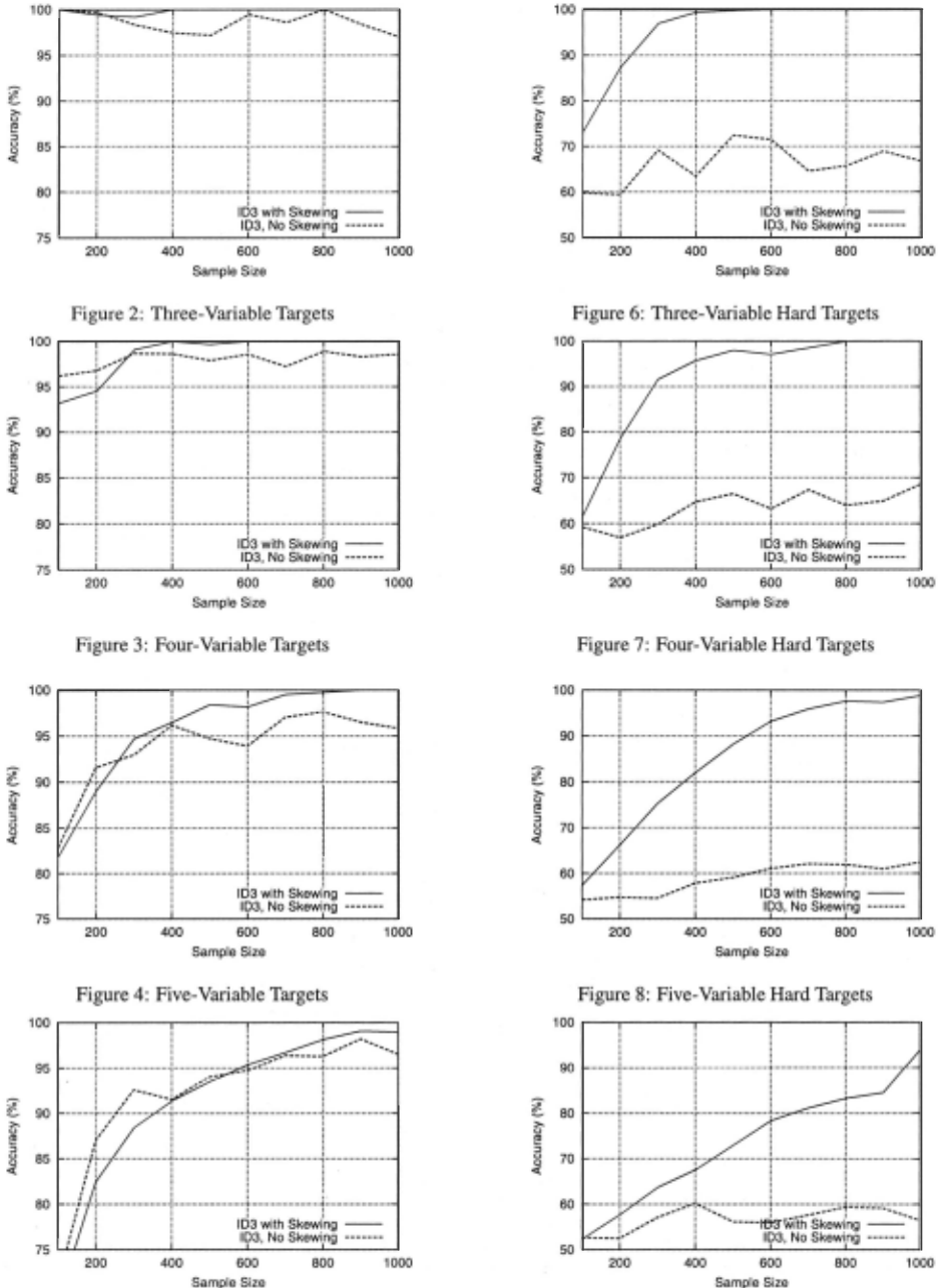
Figure 9: Six-Variable Hard Targets
| Data Set | Standard ID3 | ID3 with Skewing |
|---|---|---|
| Heart | 71.9 | 74.5 |
| Voting | 94.0 | 94.2 |
| Voting-2 | 87.4 | 88.6 |
| Contra | 60.4 | 61.5 |
| Monks-! | 92.6 | 100.0 |
| Monks-2 | 86.5 | 89.3 |
| Monks-3 | 89.8 | 91.7 |
We observe that if the target is a problematic function, skewing outperforms standard ID3 by a wide margin. The difference in accuracy was statistically significant- the 95% confidence intervals around each sample point in these graphs do not overlap once the sample sizes become moderately large. We repeated the experiment with 6-variable hard tar gets with 5000 examples to verify that skewing did indeed achieve 100% accuracy (in our noise-free setting) in this case. We also verified this behavior for 7 and 8 variable targets.
In addition to the preceding experiments, we also com pared ID3 against ID3 with skewing on several data sets in the UCI machine learning repository [Blake and Merz, 1998] us ing 5-fold cross validation. For these data sets, we discretized continuous variables by binning. Further, nominal variables were binarized using the standard 1-of-N representation. The results of these experiments appear in Table 5. In this case, we do not know whether the target concepts involve problem atic subfunctions except for the concepts in the Monk's prob lems, where the first two involve problematic subfunctions. The only task for which there is a significant difference in ac curacy is the first Monk's problem, which has an exclusive-or subfunction. We believe the reason ID3 with skewing does not dramatically outperform ID3 on the second Monk's prob lem is that the number of training instances is small ( 169) rel ative to the target function. We verified this by constructing a larger data set of 2000 examples using the concept that gen erated this data. In this case, skewing achieves an accuracy of 95%, while standard ID3 achieves 80%.
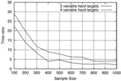
In the experiments reported in Figures 2-5, the run-time for ID3 with skewing was on average a constant times the run-time for ordinary ID3, regardless of sample size or target size. This constant was (roughly) equal to our value forT in Algorithm 1, 30. In the experiments involving hard targets, we observed that as sample size increased, ID3 with skewing became more efficient relative to ID3. This can be explained by the fact that though it takes more time to choose a split, ID3 with skewing chooses many fewer splits when the target is a hard function. In this case, the constant-factor overhead for skewing is significantly smaller than T. This behavior is shown in Figure 10. Thus in all cases, provided the sample is sufficiently large, skewing provides benefits similar to looka head, but with only a constant increase in run-time. This is the primary result of the paper.
6 Related Work
A natural question to ask of the preceding results is whether they could as easily be obtained by other techniques that ef fectively re-weight the data. We know of two such related techniques: boosting [Freund and Schapire, 1997] and bag ging [Breiman, 1996] (sampling with replacement may be thought of as providing a re-weighting of the data) .While these techniques were not developed to enable tree induc tion algorithms to address problematic functions, it is pos sible that their re-weighting schemes might nevertheless be successful in this task. Therefore, we ran ID3 with each of these re-weighting techniques on hard targets, using the same methodology as in the preceding section. We also ran ID3 with a procedure that randomly reweighted the data as in the data perturbation approaches of Elidan et ai[2002]. We ob served that ID3 with each of the three re-weighting schemes performed on average no better than ordinary ID3. Hence we conclude that the benefit of skewing comes from the type of re-weighting being performed, not merely from the general notion of re-weighting.
7 Conclusions and Future Work
We have shown that the advantages of lookahead for decision trees can be obtained with only a constant increase in run time, rather than a super-exponential increase, by the process of skewing. Nevertheless, the approach has limitations that need to be addressed in future work. It also has potential ap plications beyond decision trees, to be investigated in future work. The remainder of this section briefly outlines these di rections.
Decision tree induction algorithms often are applied to data sets that involve some continuous variables in addition to nominal variables only. Therefore, one direction for further work is to extend the skewing algorithm to handle continuous variables. Here we briefly outline a natural such extension that we plan to test in future work. For continuous variables, the favored value is either less or greater than the split point, rather than 0 or 1. This makes skewing trickier because we do not know ahead of time what split point will be chosen. Hence for each continuous value v that a variable x takes in the data set, we compute the probability that v will be Jess than or greater than the split point. To do this computation, we might assume the split point is drawn from a uniform dis tribution over the values that x takes in the data set. We can then reweight an example with the expected weight over all possible split points. For example, suppose we have 100 ex amples, and the favored value for a variable xis less. An ex ample that takes the tenth lowest value for x has probability 0.9 of being lower than the split point. Hence the weight of this example will get multiplied by (0.9)(2) + (0.1)(1) = 1.9.
Second, while we have demonstrated that skewing works for parity and other problematic functions of up to seven vari ables, for more variables it appears that large numbers of ex amples (at least several thousand) will be required. If the number of examples is too small relative to the size of the problematic portion of the target, then skewing can cause pre dictive accuracy to degrade somewhat, though the reason for this is not entirely clear. Hence if a data set is small it may be desirable to try both skewed and normal versions of the tree learner. In spite of this limitation, skewing makes it possible to gain the effect of five- or six- step lookahead where only 2- or perhaps 3-step lookahead was computationally feasible previously.
The third direction for future work is to address high dimensional data sets. The skewing approach may have trou ble with such data sets for the following reason. If each data point has thousands of features, then one data point is likely to get a much higher weight than all others (to have many more variables with the preferred values), merely by chance, lead ing to a model that overfits this data point. One solution may be to lessen the degree of skewing. This and other approaches should be tested on high-dimensional data sets.
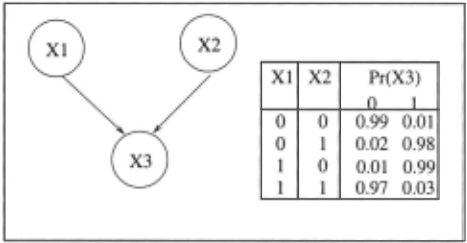
We would also like to apply the skewing approach to other types of learning algorithms that have trouble with similar hard functions. To focus on a specific algorithm for illus tration, the introduction noted that the sparse candidate algo rithm for learning Bayesian networks [Friedman et al., 1999] was susceptible to functions like exclusive-or. This suscepti bility is because of its use of information gain or more gener ally Kullback~Leibler divergence to narrow the candidate par ents for any given node. For example, suppose the variables x1 and x2 together are highly predictive of the value of x 3 and hence would be excellent parents of x3 , as shown in the Bayesian network fragment in Figure 11. If x1 and x2 are in dependent of one another and take the value 0 roughly half of the time, then among tens or hundreds of other variables nei ther x1 nor x 2 is likely to be considered as a candidate parent for x3. Nevertheless, if several skewed versions of the data are used to select candidate parents (a variable is a potential parent if it scores well according to most of the skews), then Xt and x2 are likely to be selected. Modifying the sparse can didate algorithm is an intriguing direction for further work. More generally, we believe the skewing approach presented in this paper may be applicable to a wide variety of learning algorithms, in addition to decision trees.
Acknowledgements
This work was supported in part by NSF grant 9987841, NIH grant 1R01LM07050-0l, and grants from the University of Wisconsin Graduate School and Medical School.
@inproceedings{ijcai2003p89,
  title     = {Skewing: An Efficient Alternative to Lookahead for Decision Tree Induction},
  author    = {Jr., C. David Page and Ray, Soumya},
  booktitle = {Proceedings of the Eighteenth International Joint Conference on
               Artificial Intelligence, {IJCAI-03}},
  publisher = {International Joint Conferences on Artificial Intelligence},
  editor    = {Georg Gottlob and Toby Walsh},
  pages     = {601--611},
  year      = {2003},
  url       = {https://ijcai.org/proceedings/2003/89},
}
TY - CPAPER TI - Skewing: An Efficient Alternative to Lookahead for Decision Tree Induction AU - Jr., C. David Page AU - Ray, Soumya T2 - Proceedings of the Eighteenth International Joint Conference on Artificial Intelligence, IJCAI-03 PB - International Joint Conferences on Artificial Intelligence PY - 2003 SP - 601 EP - 611 UR - https://ijcai.org/proceedings/2003/89 ER -Copied
Machine-readable versions of this paper, for tools and AI agents:





