
A Fast and Simple Algorithm for Bounds Consistency of the AllDifferent Constraint
Proceedings of the Eighteenth International Joint Conference on Artificial Intelligence. Pages 245-249.
© 2003 International Joint Conferences on Artificial Intelligence
Abstract
In constraint programming one models a problem by stating constraints on acceptable solutions. The constraint model is then usually solved by interleaving backtracking search and constraint propagation. Previous studies have demonstrated that designing special purpose constraint propagators for commonly occurring constraints can significantly improve the efficiency of a constraint programming approach. In this paper we present a fast, simple algorithm for bounds consistency propagation of the alldifferent constraint. The algorithm has the same worst case behavior as the previous best algorithm but is much faster in practice. Using a variety of benchmark and random problems, we show that our algorithm outperforms existing bounds consistency algorithms and also outperforms-on problems with an easily identifiable property-state-ofthe-art commercial implementations of propagators for stronger forms of local consistency.
- [Gabow and Tarjan, 1985] H. N. Gabow and R. E. Tarjan. A linear-time algorithm for a special case of disjoint set union. JCSS, 30(2):209-221, 1985.
- [Gent and Walsh, 1999] I. P. Gent and T. Walsh. CSPlib: A benchmark library for constraints. In CP-99, pp. 480-481 .
- [!LOGS. A., 1998] !LOG Solver 4.2 user's manual, 1998.
- [Leconte, 1996] M. Leconte. A bounds-based reduction scheme for constraints of difference. In Proc. of the Constraint-96 Int '/ Workshop on Constraint-Based Rea- soning, pp. 19-28, Key West, Florida, 1996.
- [L6pez-Ortiz eta!., 2003] A. L6pez-Ortiz, C. G. Quimper, J. Tromp and P. van Beek. Faster practical algorithms for the all-diff constraint. Technical Report, CS-2003-05, School of Computer Science, University of Waterloo, 2003.
- [Mehlhorn and Thiel, 2000] K. Mehlhorn and S. Thiel. Faster algorithms for bound-consistency of the sortedness and alldifferent constraint. In CP-2000, pp. 306-319.
- [Puget, 1998] J.-F. Puget. A fast algorithm for the bound consistency of alldiff constraints. AAAI-98, pp. 359-366.
- [Regin, 1994] J.-C. Regin. A filtering algorithm for con- straints of difference in CSPs. In AAAI-94, pp. 362-367.
- [Schulte and Stuckey, 2001] C. Schulte and P. J. Stuckey. When do bounds and domain propagation lead to the same search space. In PPDP-2001, pp. 115-126.
- [Smith eta/., 2000] B. M. Smith, K. Stergiou, and T. Walsh. Using auxiliary variables and implied constraints to model non-binary problems. In AAAI-2000, pp. 182-187.
- [Stergiou and Walsh, 1999] K. Stergiou and T. Walsh. The difference all-difference makes. In JJCAJ-99, pp. 414-419. IJCAI
- [van Hoeve, 2001] W. J. van Hoeve. The alldifferent con- straint: A survey. Submitted manuscript. Available from http:/ /www.cwi.nlrwjvhlpapers/alldiff.pdf, 2001. Link
References were extracted automatically from the PDF and may contain errors.
Full text extracted automatically from the PDF; figures, tables and equations may differ. The PDF is the version of record.
1 Introduction
Many interesting problems can be modeled and solved us ing constraint programming. In this approach one models a problem by stating constraints on acceptable solutions, where a constraint is simply a relation among several unknowns or variables, each taking a value in a given domain. The con straint model is then usually solved by interleaving backtrack ing search and constraint propagation. In constraint propaga tion the constraints are used to reduce the domains of the vari ables by ensuring that the values in their domains are locally consistent with the constraints.
Previous studies have demonstrated that designing special purpose constraint propagators for commonly occurring con straints can significantly improve the efficiency of a con straint programming approach (e.g., [Regin, 1994; Stergiou and Walsh, 1999]). In this paper we study constraint propaga tors for the alldifferent constraint. An alldifferent constraint over a set of variables states that the variables must be pair wise different. The alldifferent constraint is widely used in practice and because of its importance is offered as a builtin constraint in most, if not all, major commercial and research based constraint systems.
Several constraint propagation algorithms for the alldiffer ent constraint have been developed, ranging from weaker to stronger forms of local consistency (see [van Hoeve, 2001] for an excellent survey). Regin [1994] gives an 0( n 2 · 5 ) algo rithm for domain consistency of the alldifferent constraint, where n is the number of variables, that is based on re lating all different constraints to matchings. Leconte [ 1996] gives an O(n 2 ) algorithm for range consistency, a weaker form of consistency than domain consistency, that is based on identifying Hall intervals. Puget [1998], building upon the work of Leconte [ 1996], gives an 0 ( n log n) algorithm for bounds consistency, which is in tum a weaker form of lo cal consistency than range consistency. Mehlhorn and Thiel [2000], building upon the work of Regin, give an algorithm for bounds consistency that is O(n) plus the time needed to sort the bounds of the domains, and thus has the same worst case behavior as Puget's algorithm in the general case.
In this paper we present a fast and simple algorithm for bounds consistency propagation of the alldifferent constraint. The algorithm has the same worst case behavior as the previ ous best algorithm but is much faster in practice. Using a vari ety of benchmark and random problems, we show that our al gorithm outperforms existing bounds consistency algorithms and also outperforms-on problems with an easily identifi able property-state-of-the-art commercial implementations of propagators for stronger forms of local consistency.
A longer version of the paper containing proofs and addi tional experimentation is available [L6pez-Ortiz eta!., 2003].
2 Background
A constraint satisfaction problem ( CSP) consists of a set of n variables, {XI, ... , xn}; a finite domain dom(x;) of possible values for each variable x; and a collection of m constraints, {C1. ... , Cm}. Each constraint Cis a constraint over some set of variables, denoted by vars (C), that specifies the al lowed combinations of values for the variables in vars(C). Given a constraint C, we use the notation t E C to denote a tuple t-an assignment of a value to each of the variables in vars(C)-that satisfies the constraint C. We use the notation t [ x] to denote the value assigned to variable x by the tuple t. A solution to a CSP is an assignment of a value to each variable that satisfies all of the constraints.
We assume in this paper that the domains are totally or dered. The minimum and maximum values in the domain dam ( x) of a variable x are denoted by min( dam ( x)) and max(dam(x)), and the interval notation [a, b] is used as a shorthand for the set of values {a, a+ 1, ... , b}.
CSPs are usually solved by interleaving backtracking search and constraint propagation. During the backtracking search when a variable is assigned a value, constraint prop agation ensures that the values in the domains of the unas signed variables are "locally consistent" with the constraints.
Definition I (Support) Given a constraint C, a value a E dam ( x) for a variable x E vars (C) has: (i) a domain support inC if there exists at E C such that a = t[x] and t[y] E dam(y), for every y E vars(C); and (ii) an interval support inC if there exists at E C such that a = t[x] and t[y] E [min(dam(y)) , max(dam(y)], for every y E vars(C) .
Definition 2 (Local Consistency) A constraint C is: (i) bounds consistent iffor each x E vars (C), each of the values min(dam(x)) and max(dam(x)) has an interval support in C; (ii) range consistent iffor each x E vars(C), each value a E dam(x) has an interval support inC; and (iii) domain consistent if for each x E vars (C), each value a E dam ( x) has a domain support in C.
A CSP can be made locally consistent by repeatedly re moving unsupported values from the domains of its variables.
Example I (Puget (1998)) Consider the CSP with six vari ables x11 ··· , x6 ; with the following domains, x1 E [3, 4], x2 E [2, 4], x3 E [3, 4], x4 E [2, 5], x5 E [3, 6], and x6 E [1, 6]; and a single constraint alldifferent(x1, ... , x5). Enforcing bounds consistency on the constraint reduces the domains of the variables as follows: x1 E [3, 4], x2 E [2], x3 E [3, 4], x4 E [5], x5 E [6], and x6 E [1].
Given an alldifferent constraint over n variables, where each of the variables x;, 1 < i < n, has an interval domain dam(x;) = [min;, max;], our task is to make the constraint bounds consistent. More precisely, we must update the do main of each variable x; to dam'(x;) = [mit\, ma~], the minimum and maximum value with interval support, or re port that no solution exists.
3 Our result
In this section we present our algorithm for bounds consis tency propagation of the alldifferent constraint and analyze its worst-case complexity.
3.1 Finding Hall intervals
Following Leconte [1996] and Puget [1998], we analyze the task in terms of Hall intervals. An interval I is a Hall interval if its size equals the number of variables whose domain is contained in I . Clearly, any solution must use all the values in I for those variables, making these values unavailable for any other variable. Puget shows that an algorithm for updating lower bounds can also be used to update upper bounds. The lower bound for variable x; gets updated where min: 2: b+ 1, whenever a Hall interval [a, b] with a ::; min; ::; b < max; is found. This condition implies that any Hall interval [a', b]
with a' < a causes the same update. Thus, for the purpose of updating lower bounds, it suffices to restrict attention to left maximal Hall intervals: those [a, b] for which a is minimal.
Puget's algorithm first sorts the variables in increasing or der of max;. We assume for convenience that max; ::; maxj, fori < j. The algorithm then processes each of the variables in tum, maintaining a set of counters which count how many of the variables processed so far have a minimum bound of at least k. More precise! y, after processing x;, the counter 4 denotes the cardinality of the set {j ::; i : mini 2: k}. The algorithm stores the counters in a balanced binary tree, allowing updates in 0 (log n) time per variable.
Conceptually, our algorithm is similar to Puget's. The dif ference is in the maintenance of the counters. The key observation is that not all counters are relevant. .
Define vt = max; + 1 - k - ci as the capacity of k after processing x;. Intuitively this corresponds to as of yet unused values in the current interval.
If vi = 0 and k ::; max; then we have ci equal to the cardinality of interval [k, max;], which is thus recognized as a Hall interval. Capacities increase when maxi+1 > max; and decrease when min;+1 2: k. More precisely, from the definition of capacity we have, v~+ 1 -vi = max;+l-max; (c~+1- ci}. Note that c~+ 1 is the cardinality of the set {j ::; i + 1 : mini 2: k} = {j ::; i : mini 2: k} U {j = i + 1 : minj 2: k}) = ci + o, where o = 1 if k ::; min;+t and 0 otherwise. Hence,
Lemma I (Domination) Let k < k'. If vi ::; v~, then v[ < v[, for any i' > i.
Capacity v~, is dominated by v~ in the sense that the former cannot reach 0 before the latter, and if both reach 0, then the Hall interval starting at k' is not left-maximal. If k is not equal to any min;, then it is always dominated.by the next greater min;, hence we need only remember capacities for which k equals some min;. The critical set C is the set of such indices of undominated capacities. This set starts out as C 0 = U{min;} and becomes smaller over time as variables are processed and capacities become dominated. We denote by ci the critical set after processing X;. The next lemma shows that we can effectively test when each particular ca pacity v~ becomes zero or negative.
Lemma 2 (Zero Test) Let k, l E Ci be successive critical in dices, such that k ::; min; < l and let d = vi - vf be their difference in capacity. Suppose that for all min; < m < max;, capacity v~ 2: 0. Then when v~ is positive we ha~ max; + 1 - l + d 2: 2 and when v~ is zero or negative we have v~ = max; + 1 - l + d.
Our algorithm maintains the critical set C as a linked list in which each index points back to the preceding one. The update rule (Equation 1) increases all capacities v~- 1 , k > min;, by a certain amount, namely, max;+1 - max;- 8, and all capacities v~- 1 , k ::; min;, by 1 less than that amount.
This means that differences between adjacent critical capaci ties remain constant, except in one place: between capacities vk and vl of the ZeroTest Lemma, where the difference is re duced by 1. Therefore, testing for a zero or negative capacity need only be done at this vk. Our linked list data structure is designed to perform this operation efficiently. All dominated indices form forests pointing toward the next critical index. A dummy index at the end, which never becomes dominated (3 larger than the largest max suffices), ensures that every dom inated index has a critical one to point to. When a difference in capacity, say between indices ki < k2, is reduced from 1 to 0, k2 becomes dominated. It must then point to the next critical index, say k3 , which instead of pointing to k2 must now point to ki .
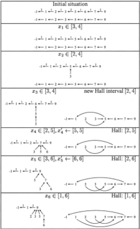
Example 2 Consider the CSP introduced in Example 1. The variables are ordered by non-decreasing max. After placing a final dummy index at 9, we get initial capacities (relative to max = 4) of v~ = 4, v~ = 3, v~ = 2, vg = -4. We represent this with the data structure 1 ~ 2 ~ 3 ? 9, which tracks the differences between adjacent critical capac ities. Initially, these are the differences between the indices themselves. Processing Xi E [3, 4] reduces the difference i i 5 between v3 and v9 from 6 to 5: 1 f-- 2 f-- 3 f-- 9. Processing x2 E [2, 4] reduces the difference between v2 and v3 from 1 to 0, causing v3 to become dominated by v2 : 1 ~ 2 ~ 9. Processing x3 E [3, 4] reduces the difi 4 ference between v2 and v9 from 5 to 4: 1 f-- 2 f-- 9. The zero capacity v2 = max + 1 - 9 + 4 = 0 signals a Hall interval [2, max] = [2, 4]. Processing x4 E [2, 5] increases max to 5 while reducing the difference between i 3 v2 and v9 from 4 to 3: 1 f-- 2 f-- 9. The zero capacity v2 = max + 1 - 9 + 3 = 0 signals a Hall interval [2, max] = [2, 5]. Processing x 5 E [3, 6] increases max to 6 while reducing the difference between v2 and v9 from 3 to 2: 1 ~ 2 ~ 9. The zero capacity v2 = max+ 1 - 9 + 2 = 0 signals a Hall interval [2, max] = [2, 6]. Finally, processing x6 E [1, 6] reduces the difference between vi and v2 from 1 to 0, causing v2 to become dominated by vi: 1 ~ 9. The zero capacity vi =max+ 1-9+2 = 0 signals a Hall interval [1, max]= [1 , 6].
3.2 Updating bounds
Finding Hall intervals is only part of the solution. We also need to efficiently update the bounds. For this we use another linked list structure, in which indices inside a Hall interval point to the location representing its upper end, while those outside of any Hall interval point left toward the next such index. We store the list of bounds in a sorted array named bounds. Intervals are hereafter numbered by their order of occurrence in this array. The linked list is implemented as an array t using indices to the bounds as pointers. The differences between critical capacities appearing above the arrows in Example 2 are stored in an array d. The algorithm shown in Figure I solves one half of the problem: updating all lower bounds. Variable n holds the number of intervals,
for i {-- 1 to nb + 1 do l t[i] {-- h[i] {-- i- 1 d[i] {-- bounds[i] - bounds[i- l] fori {-- 0 to niv - 1 do x {-- maxsorted[i].minrank y {-- maxsorted[i].maxrank z {-- pathmax(t, x + 1) j {-- t[z] d[z] {-- d[z]- 1 if d[z] = 0 then l t[z] {-- z + 1 z {-- pathmax (t, t[z]l t[z] {-- j pathset (t, x + 1, z, z ) if d[z] < bounds[z]- bounds[y] then L return Failure if h[x] > x then l w {-- pathmax (h, h[x]) maxsorted[i].min {-- bounds[w] pathset (h, x, w, w) if d[z] = bounds[z]- bounds[y] then l pathset (h, h[y], j- 1, y) h[y] {-- j- 1Algorithm 1: Algorithm for updating lower bounds.
while nb holds the number of unique bounds. The algorithm uses the following arrays:
- maxsorted [0 .. n-11: holds intervals sorted by max.
- bounds [O .. nb+1l: sorted array of min's and max's.
- t [ 0 .. nb+ 11: holds the critical capacity pointers; that is, t [ i l points to the predecessor of i in the bounds list.
- d [ 0 .. nb+ 11 holds the differences between critical ca pacities; i.e., the difference of capacities between inter val i and its predecessor in t viz. t [ i l .
- h [ o .. nb+ 11 holds the Hall interval pointers; i.e., if h [il < i then the half-open interval [bounds [h [ill, bounds [ i l) forms a Hall interval, and otherwise holds a pointer to the Hall interval it belongs to. This Hall in terval is represented by a tree, with the root containing the value of its right end.
The algorithm uses two functions for retrieving/updating pointer information, namely: pa thmax (a, x) which fol lows the chain x, a [xl, a [a [xll, ... , until it stops increas ing, returning the maximum found and pa thset (a, x, y, z) which sets each of the entries a [xl, a [a [xll, ... , a [wl to z, where w is such that a [wl equals y. The values minrank and maxrank give the index in array bounds of the min and (max+ 1) of an interval.
The algorithm examines each interval in turn, sorted by their upper bounds. It then updates capacities accordingly, followed by path compression operations on the underlying data structures. At each step we test for failure (a negative capacity) or a newly discovered Hall interval (a zero capacity, which indicates that the width of the interval is equal to the number of variables whose domain falls within that interval).
Example 3 Table 1 shows a trace of the algorithm for updat ing lower bounds (Figure 1) when applied to the CSP from Examples 1 & 2. Each row represents an iteration where a variable is processed. In the first graph the nodes are the el ements of the vector bounds. The arrows illustrate the con tent of the vector t and the numbers over them are given by the vector d. The nodes of the second graph are also the val ues found in vector bounds but the arrows are given by the vector h that keeps track of the Hall intervals.
3.3 Time complexity
The running time of the algorithm is dominated by the various calls to pathmax and pathset. Since each chain followed in a pathmax call is also followed in a subsequent path set call, we can restrict our analysis to the time spent in the latter. Consider the right-running chains in array t . Lemma 3 shows that all but a logarithmic number of indices see a rise in value as a result of a path compression operation.
Lemma 3 For any increasing sequence 0 < i 1 < i 2 < · · · < ik < n there are at most log n elements ij such that llog(ik ii)J = llog(ii+l- ii)J.
This implies that a linear number of path compressions take at most O(n log n) steps. The situation with array his similar. It follows then that the algorithm runs in time 0 ( n log n) .
The theoretical performance of the algorithm can be im proved further by observing that the union operations are al ways performed over sets whose bounds appear consecutively in a left to right ordering. This is known as the interval union find problem. Gabow and Tarjan [1985] gave a linear time solution in a RAM computer provided that the keys fit in a single word of memory. This is a reasonable assumption in current architectures with 32 or 64 bit words. Using this technique we obtain a linear time algorithm which matches the theoretical performance of Mehlhorn and Thiel's solution. We implemented this algorithm on the Intel x386 architec ture using direct assembly code calls from a C++ program. However, in practice, the O(n log n) solution outperformed both Mehlhorn and Thiel's algorithm and the algorithm using the interval union find data structure (see [L6pez-Ortiz et al., 2003] for additional discussion).
4 Experimental results
We implemented our new bounds consistency algorithm (de noted hereafter as BC) and Mehlhorn and Thiel's bounds con sistency algorithm (denoted MT) using the ILOG Solver C++ library, Version 4.2 [ILOG S. A., 1998] 1 . The ILOG Solver already provides implementations of Leconte's range consis tency algorithm (denoted RC), Regin's domain consistency algorithm (denoted DC), and an algorithm that simply re moves the value of an instantiated variable from the domains of the remaining variables (denoted as VC, for value consis tency). To compare against Puget's bounds consistency algo rithm, we use the runtime results reported by Puget [1998] for RC and our own runtime results for RC as calibration points. We believe this is valid as Puget also uses a similar vintage of ILOG Solver and when we compared, we were careful to use the same constraint models and variable orderings.
We compared the algorithms experimentally on various benchmark and random problems. All the experiments were run on a 300 MHz Pentium II with 228 MB of main memory. Each reported runtime is the average of 10 runs except for random problems where 100 runs were performed.
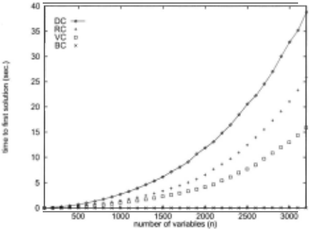
We first consider a problem introduced by Puget ([1998]; denoted here as Pathological problems) that were "designed to show the worst case behavior of each algorithm". A Patho logical problem consists of a single alldifferent constraint over 2n + 1 variables with dom(x;) =[i-n, 0], 0::; i::; n, anddom(x;) = [O,i-n],n+l::; i::; 2n. Theproblemswere solved using the lexicographic variable ordering. Here, our BC propagator offers a clear performance improvement over propagators for stronger forms of local consistency (see Fig ure 1). Comparing against the best previous bounds consis tency algorithms, our BC propagator is approx. 2 times faster than MT and, using RC as our calibration point to compare against the experimental results reported by Puget [ 1998], ap prox. 5 times faster than Puget's algorithm.
1 The code discussed in this section is available on request from vanbeek@uwaterloo.ca
We next consider the Golomb ruler problem (see [Gent and Walsh, 1999], Problem 6). Following Smith et al. [2000] we modeled the problem using auxiliary variables (their "ternary and all-different model") and we used the lexicographic vari able ordering. This appears to be the same model as Puget [ 1998] uses in his experiments as the number of fails for each problem and each propagator are the same. Here, our BC propagator is approximately 1.6 times faster than the next fastest propagator used in our experiments (see Table 2) and, again using RC as our calibration point, approximately 1.5 times faster than Puget's bounds consistency algorithm.
| m | vc | RC | DC | MT | BC |
|---|---|---|---|---|---|
| 8 | 0.9 | 0.5 | 0.6 | 0.6 | 0.3 |
| 9 | 9.0 | 3.8 | 4.6 | 4.4 | 2.3 |
| 10 | 87.3 | 31.7 | 39.5 | 36.5 | 18.9 |
| 11 | 1773.6 | 688.1 | 871.2 | 841.4 | 437.6 |
We next consider instruction scheduling problems for single-issue processors with arbitrary latencies. Instruction scheduling is one of the most important steps for improv ing the performance of object code produced by a compiler. Briefly, in the model for these problems there are n variables, one for each instruction to be scheduled, latency constraints of the form x; ~ Xj + d where dis some small integer value, a single alldifferent constraint over all n variables, and re dundant constraints called "distance constraints" In our ex periments, we used fifteen representative hard problems that were taken from the SPEC95 floating point, SPEC2000 float ing point and MediaBench benchmarks. The minimum domain size variable ordering heuristic was used in the search (see Table 3). On these problem too, our BC propagator offers a clear performance improvement over the other propagators.
| n | vc | RC | DC | MT | BC |
|---|---|---|---|---|---|
| 69 | 0.02 | 0.04 | 0.04 | 0.02 | |
| 70 | 0.02 | 0.05 | 0.04 | 0.02 | |
| Ill | 0.08 | 0.07 | 0.12 | O.li | 0.07 |
| 211 | |||||
| 2I4 | 40.64 | 0.67 | 1.20 | 0.94 | 0.46 |
| 216 | 0.3I | 1.08 | 0.72 | 0.38 | |
| 220 | 0.29 | 0.93 | 0.66 | 0.32 | |
| 377 | 0.84 | 3.94 | 2.41 | 0.79 | |
| 381 | 0.28 | 0.50 | 3.18 | 1.15 | 0.39 |
| 394 | 2.66 | 7.15 | 2.66 | 1.65 | |
| 556 | |||||
| 690 | 1.91 | 26.88 | 3.95 | 1.61 | |
| 69I | 14.47 | 40.50 | 6.30 | 3.I4 | |
| 856 | 7.72 | 17.09 | 10.86 | 5.48 | |
| 1006 | 10.35 | 87.23 | I5.90 | 5.95 |
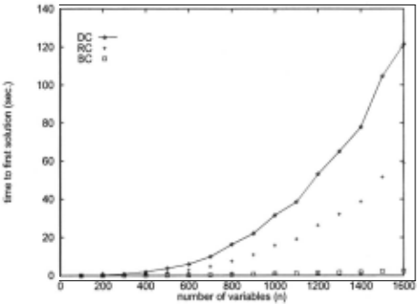
To systematically study the scaling behavior of the algo rithms, we next consider random problems. The problems consisted of a single alldifferent constraint over n variables and each variable x; had its initial domain set to [a, b], where a and b, a< b, were chosen uniformly at random from [1, n] . The problems were solved using the lexicographic variable ordering. In these "pure" problems nearly all of the run-time is due to the alldifferent propagators, and one can clearly see the quadratic behavior of the RC and DC propagators and the nearly linear incremental behavior of the BC propagator (see Figure 2). On these problems, VC (not shown) could not solve even the smallest problems ( n = I 00) within a 10 minute time bound and MT (also not shown) was 2.5-3 times slower than our BC propagator.
Having demonstrated the practicality of our algorithm, we next study the limits of its applicability. Schulte and Stuckey [2001] investigate cases where it can be proven a priori that maintaining bounds consistency during the search, rather than a stronger form of local consistency such as do main consistency, does not increase the size of the search space. The Golomb ruler problem is one such example. In general, of course, this is not the case and using bounds con sistency can exponentially increase the search space.
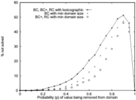
To systematically study the range of applicability of the al gorithms, we next consider random problems with holes in the domains of the variables. The problems consisted of a single alldifferent constraint over n variables. The domain of each variable was set in two steps. First, the initial domain of the variable was set to [a, b], where a and b, a ~ b, were chosen uniformly at random from [1, n]. Second, each of the values a+ 1, . .. , b-l is removed from the domain with some given probability p. The resulting problems were then solved using both the lexicographic and the minimum domain size variable ordering heuristics. These problems are trivial for domain consistency, but not so for bounds and range consis tency. We recorded the percentage that were not solved by BC and RC within a fixed time bound (see Figure 3). If there are no holes in the domains of the variables, then bounds con sistency is equivalent to range and domain consistency. As the number of holes increases, the performance of bounds and range consistency decreases and they become less ap propriate choices. The range of applicability of BC can be extended somewhat following a suggestion by Puget [1998] of combining bounds consistency with value consistency (de noted as BC+ and MT+). On these problems, BC, BC+, and RC are theoretically equivalent when using the lexicographic variable ordering and BC+ and RC are experimentally equiv alent when using minimum domain (see Figure 3).
We also performed experiments on n-queens, quasigroup existence, and sport league scheduling problems. Interest ingly, in these experiments, RC was never the propagator of choice. On problems where holes arise in the domains, DC was the best choice (except for on n-queens problems, where VC was considerably faster), and on problems where holes do not arise in the domains, BC was the clear best choice. Clearly, whether the domains have holes in them is a prop erty that is easily identified and tracked during the search. Thus, the best choice of propagator could be automatically selected, rather than left to the constraint modeler to specify as is currently the case.
5 Conclusions
We presented an improved bounds consistency constraint propagation algorithm for the important alldifferent con straint. Using a variety of benchmark and random problems, we showed that our algorithm significantly outperforms the previous best bounds consistency algorithms for this con straint and can also significantly outperform propagators for stronger forms of local consistency.
Acknowledgements
We thank Kent Wilken for providing the instruction schedul ing problems used in our experiments.
@inproceedings{ijcai2003p36,
  title     = {A Fast and Simple Algorithm for Bounds Consistency of the AllDifferent Constraint},
  author    = {López-Ortiz, Alejandro and Quimper, Claude-Guy and Tromp, John and van Beek, Peter},
  booktitle = {Proceedings of the Eighteenth International Joint Conference on
               Artificial Intelligence, {IJCAI-03}},
  publisher = {International Joint Conferences on Artificial Intelligence},
  editor    = {Georg Gottlob and Toby Walsh},
  pages     = {245--249},
  year      = {2003},
  url       = {https://ijcai.org/proceedings/2003/36},
}
TY - CPAPER TI - A Fast and Simple Algorithm for Bounds Consistency of the AllDifferent Constraint AU - López-Ortiz, Alejandro AU - Quimper, Claude-Guy AU - Tromp, John AU - van Beek, Peter T2 - Proceedings of the Eighteenth International Joint Conference on Artificial Intelligence, IJCAI-03 PB - International Joint Conferences on Artificial Intelligence PY - 2003 SP - 245 EP - 249 UR - https://ijcai.org/proceedings/2003/36 ER -Copied
Machine-readable versions of this paper, for tools and AI agents:





