
Use of Off-line Dynamic Programming for Efficient Image Interpretation
Proceedings of the Eighteenth International Joint Conference on Artificial Intelligence. Pages 1319-1324.
© 2003 International Joint Conferences on Artificial Intelligence
Abstract
An interpretation system finds the likely mappings from portions of an image to real-world objects. An interpretation policy specifies when to apply which imaging operator, to which portion of the image, during every stage of interpretation. Earlier results compared a number of policies, and demonstrated that policies that select operators which maximize the information gain per cost, worked most effectively. However, those policies are myopic- they rank the operators based only on their immediate rewards. This can lead to inferior overall results: it may be better to use a relatively expensive operator first, if that operator provides information that will significantly reduce the cost of the subsequent operators. This suggests using some lookahead process to compute the quality for operators non-myopically. Unfortunately, this is prohibitively expensive for most domains, especially for domains that have a large number of complex states. We therefore use ideas from reinforcement learning to compute the utility of each operator sequence. In particular, our system first uses dynamic programming, over abstract simplifications of interpretation states, to precompute the utility of each relevant sequence. It does this off-line, over a training sample of images. At run time, our interpretation system uses these estimates to decide when to use which imaging operator. Our empirical results, in the challenging realworld domain of face recognition, demonstrate that this approach works more effectively than myopic approaches.
- J. Bins B. Draper and K. Baek. Adore: Adaptive object recognition. In Videre, 1(4), pages 86-99,2000.
- C Boutilier, T Dean, and S Hanks. Decision- theoretic planning: Structural assumptions and computa- tional leverage. J. Artificial Intelligence Reseach, 1999.
- V Bulitko, B Draper, and I. Levner. MR ADORE control policies. TR, Dept. of Computing Science, U. of Alberta, 2002.
- R.O. Duda and P.E. Hart. Pattern Classification and Scene Analysis. Wiley, New York, 1973.
- K Etemad and R Chellappa. Discriminant analysis for recognition of human faces. J. Optical Society of America, 1997.
- R Huang and S Russell. Object identification: A bayesian analysis with application to traffic surveillance. Artificial Intelligence, 1996.
- R. Isukapalli and R. Greiner. Efficient car recognition policies. In ICRA, pages 2134-2139, Seoul, 2001.
- I GO 1
- R. Isukapalli and R. Greiner. Efficient interpretation policies. In IJCAJ, Seattle, 2001. IJCAI
- T M Mitchell. Machine Learning. McGraw-Hill, 1997.
- A R Pope and D Lowe. Learning object recognition models from images. In Early Visual Learning, 1995.
- A Pentland, B Moghaddam, and T Stamer. View- based and modular eigenspaces for face recognition. In IEEE CVPR, 1994.
- P Phillips, H Wechsler, J Huang, and P Rauss. The feret database and evaluation procedure for face recog- nition algorithms. Image and Vision Computing, 1998.
- R. S. Sutton and A. G. Barto. Reinforcement Learn- ing: An Introduction. MIT Press, Cambridge, 1998.
- M Turk and A Pentland. Eigenfaces for recognition. J. Cognitive Neuroscience, 1991.
References were extracted automatically from the PDF and may contain errors.
Full text extracted automatically from the PDF; figures, tables and equations may differ. The PDF is the version of record.
1 Introduction
Interpretation is the process of finding the likely mapping from portions of an image to real-world objects. It is the ba sis for a number of imaging tasks, including recognition ("is objectX in the image?") and identification ("which object is in the image?"), as well as several forms of tracking ("find all moving objects of typeX in this sequence of images"), etc. [PL95; HR96]. It is important that an interpretation sys tem (IS) be efficient as well as accurate. Any IS should have
Russell Greiner
Department of Computing Science University of Alberta Edmonton, AB T6G 2E8 Canada greiner@cs.ualberta.ca
access to an inventory of "imaging operators" -like edge de tectors, region growers, corner locators, etc., each of which, when applied to any portion of the image, returns meaningful tokens (like circles, regions ofthe same color, etc.). An "inter pretation policy" specifies which operator to apply to which portion of the image, during each step of the interpretation process. Such policies must, of course, specify the details: perhaps by specifying exactly which bottom-up operators to use, and over what portion of the image, if and when to switch from bottom-up to top-down, which aspects of the model to seek, etc.
Our earlier work [IGOl b] considered various types of poli cies, towards demonstrating that an "information theoretic policy", which selects operators that maximize the informa tion gain per unit cost of the imaging operator, work more ef fectively than others. However, the [IGOl b] policies evalu ate each operator o( ·) myopically - i.e., independent of the cost and effectiveness of subsequent operators that would be applied, after performing this o( ·). To see why this is prob lematic, assume the task is to determine whether there is an airplane in an image, by seeking the various parts of an air plane- e.g., the fuselage, wings, engine pods, tailpiece, etc. Now consider the Oep operator that detects and locates the en gine pods. As the engine pods are small and often partially occluded, Oep is probably expensive. However, once these parts have been located, we expect to find the associated wings very easily, and then the remaining parts required to identify the entire airplane. A myopic policy, which evaluates an oper ator based only on its immediate cost, would miss this connec tion, and so would probably prefer a cheaper operator over the expensive Oep· A better policy would consider "operator in teractions" (here, relating Oep to (say) the "wing finder opera tor") when deciding which operator to apply. The data in Sec tion 5 (related to the complex task of face recognition) shows that such non-myopic policies can be both more accurate, and more efficient.
Of course, non-myopic policies must use some type of lookahead to evaluate the quality of its operators; this can be combinatorially expensive to compute. We address this con cern by (1) dealing with an abstract version of the "interpreta tion state space", and then by (2) using dynamic programming techniques over this abstracted space, pre-computing many relevant "utility" [SB98] values off-line [BDBOO]. In partic ular, our system computes the utility of imaging operator sequences in each state s encountered, based on data from a set of training examples. It produces a policy, which maps each state s to the operator o; that appears to be the most promis ing, incorporating this lookahead. At run-time, our system finds the best matching state and applies the operator associ ated with that situation. Our empirical results, in the domain of face recognition, show that such policies work effectively - better than the best results obtained by any of the earlier myopic systems.
Section 2 presents relevant related work, to help frame our contributions. Section 3 discusses the salient features of inter pretation strategies. Section 4 then presents our approach, of using reinforcement learning in image interpretation, within the domain of face recognition, using operators that each cor respond to types of eigenfeatures. Section 5 provides empiri cal results that support our claims.
2 Related work
We produce an interpretation of an image by applying a se quence of operators, where each operator maps the current state (typically a partial interpretation) to a new state. As the effects of an operator may depend on information not explic itly contained in the state description, this mapping is stochas tic. Moreover, each operator has a cost, and the state associ ated with the final interpretation has a "quality" (i.e., its ac curacy as an interpretation). As such, we view this image interpretation task as a "Markov Decision Problem" (MDP). This means we can apply the host of reinforcement learning techniques [SB98] to this problem. This specific application area, of image interpretation, follows the pioneering work of Draper [BDBOO], which shows that dynamic control policies can outperform hand-coded policies. We extend their work by addressing and exploiting the issue of operator interactions and by doing a systematic analysis of the cost and accuracy tradeoffs in face recognition.
While we could encode each state as the entire image, this would be too unwieldy. Boutilier et a!. [BDH99] survey sev eral types of representations in planning problems and discuss ways to exploit them to ease the computational cost of policies or plans. Their work focuses on abstraction, aggregation and decomposition techniques. We use abstractions to reduce the size of each state, and hence of the state space we are explor ing; moreover, we are not concerned with the general plan ning problem. Our system is similar to the "forest inventory management system" [BDL02]. In their system, the output of some operators provide the input to some other operator, while in our system the result of one operator is used to nar row the search for some other operator. Moreover, our sys tem can exploit the structure specific to our task to bound the lookahead depth.
3 Framework
As suggested above, our overall objective is to produce an ef fective interpretation policy- e.g., one that efficiently returns a sufficiently accurate interpretation, where accuracy and ef ficiency are each measured with respect to the underlying task and the distribution of images that will be encountered. This section makes this framework more precise. Subsection 3.1
specifies our particular task; Subsection 3.2 lists the strategies we will evaluate; Subsection 3.3 outlines our performance do main, face recognition; and Subsection 3.4 describes the spe cific operators we will use.
3.1 Input to the Interpretation System
We assume that our interpretation system "IS" is given the fol lowing information:
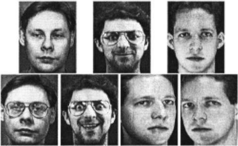
* The distribution D of images that the IS will encounter, encoded in terms of the distribution of objects and views that will be seen, etc. For our face recognition task, this corre sponds to the distribution of all people the system will see, which varies over race, gender and age, as well as poses and sizes. We approximate this using the images given in the training set. See Figure 1. ·
* The task T = (V; Cmax, Pmin) includes two parts: First, V specifies the objects that the IS should seek, and what IS should return. Second, the task specification also provides the "evaluation criteria" for any policy, which is based on both the expected "accuracy" (P min) and the maximum interpreta tion "cost" (Cmax), which the IS should not exceed.
Here, V specifies our task is to identify the person from his/her given test image (wrt the people included in the train ing set), subject to the accuracy Pmin and cost requirements Cmax·
* The set of possible "operators" 0 = { oi} includes (say) various edge detectors, region growers, graph matchers, etc. For each operator oi, we must specify
- its input and output,
- its "effectiveness", which specifies the accuracy of the output, as a function of the input.
- its "cost", as a function of (the size of) its input and pa rameter setting.
We will use a specific set of operators in our face recognition task; we describe these in detail in Section 3.4.
Borrowing from the MDP literature, we view the main in put to each operator as its "state". As we are dealing with scenes, we could use the entire pixel image as (part of) the state. However, for reasons of efficiency, we will often use an abstracted view F( s) of (our interpretation of the) the scene s. Section 3.4 presents the specific abstraction we are using.
3.2 Strategies
Strategy INFOGAIN: selects the operator that provides the largest information gain (per unit cost) at each step. This myopic strategy first computes the expected information gain EI G( o) for each possible operator and argument combination o, as well as the cost c( o). It then executes the operator that maximizes their ratio, o* = argmax 0 { E I G ( o) / c( o)}.
We focus on this strategy as a number of earlier empirical studies have demonstrated that it was the best of all of the (my opic) strategies considered, across a number of task-contexts and domains, including simple blocks world [IGOia] , car recognition (identifying the make and model of a car based on its taillight assembly [IGOla]), as well as the face recognition system considered here [IG01b].
Strategy BESTSEQ: selects an operator o:Bs that appears to be the most promising in the current abstract state F( s ), as given by the utility o'Bs = 1r*(F( s )), where 1r* is the (opti mal) mapping from state to actions. See Section 4 for details.
3.3 Face recognition task
We investigate the efficiency and accuracy of the strategies I is ted above in the domain of face recognition [TP91; PMS94; PWHR98; EC97]. This section briefly discusses the promi nent "eigenface" technique of face recognition that forms the basis of our approach; then presents our framework, describ ing the representation and the operators we use to identify faces; and finally presents our face interpretation algorithm, for identifying a person from a given image of his/her face.
Eigenface and EigenFeature Method: Many of today's face recognition systems use Principal Component Analysis (PCA) [TP91]: Given a set of training images of faces, the system first forms the covariance matrix C of the images, then computes the k main eigenvectors of C ("eigenfaces"). Ev ery training face h; is then projected into this coordinate space ("facespace"), producing a vector 0; = [w~i), w~i), . .. , wii)J.
During recognition, the test face htest is similarly projected into the facespace, producing the vector Otest. which is then compared with each of the training faces. The best matching training face is taken to be the interpretation [TP91].
Following [PMS94], we extend this method to recognize facial features- eyes, nose, mouth, etc. -which we then use to help identify the individual in a given test image. We parti tion the training data into two sets, T = { h1,;} for construct ing the eigenfeatures and S = { h2,;} for collecting statistics, where each set contains at least one face of each of then peo ple. (Feature regions for the training data T were extracted using the operators explained in 3.4 and verified manually for correctness). Letting id(h) denote the person whose face is given by h, we have id(h1,;) = i = id(h2,i) fori = l..n; each remaining h 1,j and h2,j (j > n) also maps to l..n; i.e., id(hi ,j ),id(h2,k) E {l, ... ,n}
We use PCA on the mouth regions of each T image, to pro duce a set of eigenvectors; here eigen-mouths. For each face image h;, let o~m) be the "feature space" encoding of h/s mouth-region. We will later compare the feature space encoding o~:)t of a new image htest against these {O~m)} vectors, with the assumption that o~:~ ~ oim) suggests that htest is really person i -i.e., finding that 110~:~ - oim) II is small should suggest that id(htest) = i. (Note II · II refers to the £2 norm, aka Euclidean distance.) To quantify how strong this belief should be, we compute M = ITI x lSI values {d;,j} where each d ;, j = 110~~) - 0~~) II is the Euclidean distance between the "eigen-mouth encodings" ofT's h1,; and S's h2 ,j· Using the T training data, we can learn a mapping from these values to probabilities P( 110~:~- oim) Ill id(htest) = i ), which we can use to estimate P( o~:~ I id(htest) = i ). (See [IGOlb] for details.)
We compute similar estimates for the other facial features, such as nose (n), left eye (le) and right eye (re). We then use the Nai've-Bayes assumption [DH73] (that features are inde pendent, given a specific person) 1 to compute a cumulative
1 0f course, this assumption is alm_ost assuredly false in our sit-
"face probability" from these "feature probabilities": the val ues IIO~~~t- O~J) II for each feature f, corresponding to a set of P( o~:~ I id(htest) = i) values (one for each individual i). We then compute
where o: is a scaling constant.
3.4 Operators
We use four classes of operators, 0 {ole(k,C,r), Ore(k,C,r), On(k ,C,r), Om(k ,C,r)} to detect respectively "left eye", "right eye", "nose" and "mouth". Each specific operator also takes several pa rameters: k E {25, 30, 35, 40, 45} specifies the number of eigen-vectors being considered; the other parameters £ = (Cx, Cy) and r = ( r x, r y) specify the space this operator will sweep, looking for this feature: It will look in the rectangle (Cx ± rx, Cy ± ry); i.e., sweep rx x ry pixels, centered at (Cx, Cy)·
Each instantiated operator o( ·) E 0 takes as input the im age of a test face htest. and returns a probabilistic distribution over the individuals. It has three subtasks: SubTask#l locates the feature h~~~t from within the entire face htest· Here we use a simple template matching technique in which we search in the fixed region r of size rx x ry pixels, centered at pixel £. SubTask#2 then projects the relevant region of the test image h~~~t into the feature space- computing o~~l t of dimen sion k. SubTask#3 uses this O~~lt to compute first the values di ,test = IIO~~;t- oifl II for each person i and then to com pute the probability P( id(htest) = i I o~~lt) for each person i. We use Equation 1 to update the distribution when consid ering the 2nd and subsequent features; see [IGOlb] . For each eigenspace dimension k, we empirically determined the cost (in milliseconds) of the four operators-
where lrl = rx x ry is the size of the range. While increas ing the dimensionality k of the feature space should improve the accuracy of the result, here we see explicitly how this will increase the cost.
4 Use of Dynamic Programming
This section briefly overviews MDPs, presents "state abstrac tion" in face recognition and shows how dynamic program ming can be used to compute the utility of operators in ab stracted states. We also discuss operator interaction and de scribe how it can be exploited in face recognition.
uation. However, this classification has been found to work well in practice [Mit97] .
4.1 Markov Decision Problem
A Markov Decision Problem can be described as a 4-tuple (S, A, M, R) where S = { s1, s2, ... , sn} is a finite set of states, A {a1,a2, ... ,am} is a finite set of ac tions, M : S x A x S ---> [0, 1] is the state transition proba bility function (M:, 8 , = P( s' I s, a) is the probability that taking action a in situation s leads to being in state s') and R : S x A ---> ~ is the reward an agent gets for taking an action a E A in state s E S . The Markov property holds if the transition from state Si to s 1 using action a depends only on S i and not the previous history. A policy 1r : S ---> A is a mapping from states to actions. For any policy 1r, we can define a utility function Urr such that
which corresponds to the expected cumulative rewards of ex ecuting the apparently-optimal action a in states, then follow ing policy 1r after that.
Given an MDP, we naturally seek an optimal policy 1r* - i.e., a policy that produces the optimal cumulative reward for each state, U*(s). Dynamic programming provides a way to compute this optimal policy, by computing the utilities of the best actions. Of course, given the values of U* (·),the optimal action at each states is simply 1r* ( s) = argmaxa { R( s, a) + l:s' M~ 8 , X U*(s')}.
This can be challenging in the general setting, where se quences of actions can map one state to itself; much of the work in Reinforcement Learning [SB98] is designed to ad dress these issues. In our current case, however, we will see there is a partial order on the states, meaning no sequence of actions can map a state to itself. Here, we can use dynamic programming to compute the optimal utility for each "final step", then use these values to compute the optimal action (and utility) for each penultimate state, and so forth.
4.2 State abstraction
An MDP involves "states". In our face recognition task, any attempt to define states in terms of the pixel values of an image would be problematic, as there will be far too many states to enumerate. Following [BDBOO; BDL02], we use the notion of "abstract states", which basically redefines an original state in a much more compact form, using only the certain aspects of the state. Since we recognize a person using the features, we define an abstraction function
where s is the actual complex state as present in the image and (xi, Yi ) denotes the location (center) of feature fi (left eye, right eye, nose or mouth) in the image. (Here C is the total cost we have spent so far, and J5 = (P( id() = xI E) )x is the current posterior distribution over the possible faces, based on the current evidence E.) The location of some feature fi may not yet be known in an image; here, we use the value of -' for both Xi and Yi· Further, we say two abstractions are "8equivalent", written :F( s1 ) ;:::;jo :F( s2 ), iff
- s1 and s2 have located the same set of features- i.e., xi(sl) =-'-iff xi(s2) =-'- and
-i.e., when the distance (in pixels) between the centers of feature f i in s1 and s2 is small (:::::; 8).
As we are using normalized images that contain only faces, denoting the distance in absolute pixel values is not an issue. In general, 8 is a small, predefined constant; we used 10. 2
The result of abstraction is that a large number of complex states can be described by a small number of compact state descriptions. Of course, the same abstract state can represent multiple states- :F( s1) = :F( s2) when s1 -1- s2 .
We use a lookahead algorithm to compute the U-values. Since we consider only four features, we need a lookahead of only depth four. Moreover, we can do this during the training phase. We will use the reward function
that penalizes each operator a by a times the time t( a) it re quired (in seconds) as well as a positive score for obtaining the correct interpretation (here x* represents that correct identity of the person in the image.) We used a = 0.2. During the training phase, our system finds the optimal operator sequence -i.e., the one that has the maximum U'(s) = U(:F( s )) value, based on the abstracted state :F( s ).
4.3 Dynamic Programming
This section shows how to compute U(s) utility values.
Tree expansion: We use four classes of operators 0 {ole(k,R,r), Ore(k,R,r), On(k,R,r), om(k,R,r)}, each with 5 different values of k E {25, 30, 35, 40, 45}, for a total of 20 operators (see Section 3.4). The parameters R = (Rx, Ry) and r = (rx, ry) specify the rectangular area where the operator will search. Our system does not have to search over their values; instead, it directly computes their values from the locations of the features (h, h, ... , fi) ( i < 4) we have already detected; see Section 4.4.
Our system expands the operator tree exhaustively using a depth-first search. Of course, the depth of the tree is at most 4 (not 20), as we only consider at most one instance of each operator along any path.
Computing U( s ): We compute the various utility values us ing a dynamic programming approach:
- (i) We first apply every sequence of 4 different operators to the original image, to produce the set of all possible sC 4 ) leaf states. Then set U(sC 4 l) = P( id() = x* IE), where x* is the correct interpretation, and E is the observed locations of the various features.
- (ii) Now consider each state sC 3 ) that involves some set of 3 operators. For each, we can consider all 5 + 1 possible ac tions: either Stop, or apply the remaining operator (with one of the 5 possible k values). We can trivially compute the util ity of each option: as P( x* IE') for the Stop action, and -a t(a) + U(sC 4 l) ifthe action a takes time t(a) and produces
2 For this value of o, we found that there were about 1600 entries ofF ( s ) totally.
the state 8( 4 ). We set U ( 8( 3 ) ) to be the largest of these 6 val ues, and 1r BS ( 8( 3 ) ) to the action which produced this largest values.
After computing U( 8( 3 )) for all "depth-3" states, we then recur, to deal with depth-2 states, and so forth.
Of course, these states here actually refer only to the ab stracted state F( 8 ). Moreover, we "bin" these values: Sup pose we have encountered some abstracted state F( 8 1 ). If we later find a state 82, where F( 8 1 ) ~r5 F( 82 ), and de termine U(F( 8 1 )) < U(F( 8 2 )), we would then reset the value of U(F( 81 )) and 7rBs(F( 81 )) to be the values found for F( 82 ).
Retrieving the most promising operator during interpre tation: This entire procedure of computing the optimal policy 1r BS is done off-line, during the training phase. During inter pretation (performance phase), in any state 8i we (i) find the "nearest neighbour" F( 8j ), such that the sum of the distances between the corresponding features in F( 8i ) and F( 8j ) is the minimum over all possible entries; and (ii) return the oper ator 7rBs(F( 8j )), which is either "Stop", or an instantiated operator- say On (25, (50, 66), (60, 52) ). If not-Stop, the run-time system then executes this operator to locate another feature, which produces a new state (updating the total cost and posterior distribution as well). It then determines the next action to perform, and so forth.
There is one place where our system might perform differ ently from what the policy dictates: As we are maintaining the actual cost so far, and the actual posterior distribution over interpretations, our run-time system will actually terminate if either the actual cost has exceeded our specs, or if the highest probability is above the minimal acceptable value.
Notice, given our specific set-up- e.g., only 4 types of op erators that can only be executed once, and which always suc ceed, etc. -the policy obtained can be viewed as a "straight line" policy: seek one specific feature, than another, until achieving some termination condition; see Figure 2 for an ex ample. In general, this basic dynamic programming approach could produce more complex policies.
4.4 Operator dependencies
Our face recognition system will exploit a certain type of op erator interactions, viz., using the result of one operator to sim plify a subsequent one. That is, after detecting some feature (say the left eye), we expect to have some idea where to find Figure 2: Policy 7rBS learned by BESTSEQ, for (Cmax = 00, Pmin = 0.9)
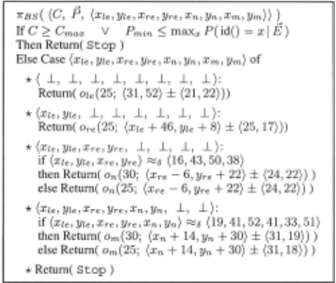
the other features (e.g., the right eye). We model this as a lin ear function, mapping from the location of the left eye to the expected location of the right eye. If the left eye was detected at (xze, Yze), then the expected location of the right eye would be the window (xze + 46, Yle + 8) ± (25, 17). We also model the "variance" - i.e., the size of the search window around this expected position. To be more precise, let us assume that the search window for some feature h is of size rx1 x ry1 pixels. After detecting feature f2, we instead search for h in a smaller region r~ 1 x r~ 1 , centered at the location that we computed from h's location, using that linear function.
After observing several features (say nose and left eye), we will have several estimates for the location of the current fea ture (here right eye). Here we take the smallest bounding box and use that as the search area for locating the current feature. This "factoring" means we need only consider a set of 4 x 3 transformations (of each of the four feature versus the other three features), rather than deal with all possible subsets.
To make these ideas more concrete: Initially, given no other information, we would look for the right eye in the region (67, 52)± (25, 22). However, after finding the left eye at loca tion Rze = (25, 50) our system knows that, if asked to look for the right eye, it should search in the region (71, 58)± (25, 17). (We are not committing to looking for the right eye at this time; just indicating where to search, if requested.) Notice this region is different from the one we would consider if we had not located the left eye; moreover, if we also knew that the nose was at location Rn = (30, 50) (as well as left eye), we would use a yet more refined region- here (61, 55) ± (15, 12).
4.5 Image interpretation policies
During interpretation, INFOGAIN and (the policy produced by) BESTSEQ each iteratively select an operator o(k) E 0. (Recall that the values of r and e are determined from the con text (of other detected features); we therefore do not need to specify them here.) INFOGAIN chooses an instantiated op erator o = ow(kw) that has the maximum EIG(o)jc(o)
value. BESTSEQ selects an operator o88 = 7rBs(F( s )) where sis the current state and 1r BS is the (optimal) mapping from state to actions. In each case, the operator is applied to the appropriate region in the given test face image and the dis tribution is updated ... until one face is identified with suffi ciently high probability(> Pmin) or the system fails (by ex hausting all the possible operators, or cost > Cmax).
5 Experiments
We used face images of 102 different people, each 92 x 112 pixels. We assigned 187 images to the set T, another 187 im ages to Sand used another 333 as test images. 3 As shown in Figure 1, the faces are more or less in the same pose (facing front), with some small variation in size and orientation. 4 We considered all 20 operators based on the four features listed above and k E {25, 30, 35, 40, 45} for each feature. The BESTSEQ interpretation policy decides precisely what oper ator oi(k, £, r) to apply on which portion of the image, given each state (which here corresponds to a specific set of infor mation gathered); see Figure 2.
Basic Experiment: We set Pmin = 0.9 and Cmax = oo (i.e., no upper limit on identification cost). 5 In each "set-up", we assigned a random probability to each person (correspond ing to drawing a sample with replacement). On each run, we picked one face randomly from the test set as the target, and identified it using each of the policies. We repeated this for a total of 30 runs per set-up, then changed the probability dis tribution and repeated the entire process again, for a total of 15 set-ups. The accuracy of identification for lNFOGAIN and BESTSEQ are 89.78% and 90.44%, respectively. (Recall both were required to obtain at least Pmin = 90%.) The average cost of identification was 1.045 ±0.038 and 0. 717 ±0.030 sec onds6 for INFOGAIN and BESTSEQ respectively. Hence, we see BESTSEQ took much less time than INFOGAIN to obtain this level of accuracy.
The first two rows of Table 1 shows how often INFOGAIN (resp., BESTSEQ) used one (resp., two, three, four) operators before terminating, over these 450 runs. We observe the IN FOGAIN applied slightly more operators than BESTSEQ on the average. More importantly, as BEST SEQ can exploit sim ple operator interactions, the search area it uses for the sub sequent operators can be narrower than lNFOGAIN's. These two factors result in a much lower cost for BESTSEQ.
Bounding the Cost: In many situations we need to impose a hard restriction on the total cost; we therefore considered var- BS = BESTSEQ; IG = lNFOGAIN
3We assume that any test face-image belongs to one of the people in the training set, but probably with a different facial expression or in a slightly different view, and perhaps with some external features not in the training image (like glasses, hat, etc.), or vice versa.
4 (1) These faces were downloaded from the web sites whi techapel. media. mit. edu and www. cam-orl. co. uk. (2) This work assumes the head has already been located and normalized; if not, we can use standard techniques [TP91] first.
5 The other part of the task, V, is "identifying people"; this is true for all of the experiments discussed here.
6 All the experiments reported in this paper were run on a Pentium 866 MHz. PC with 128MB RAM running Linux OS 2.2.19-12.
| Table 1: How often BEST SEQ (INFOGAIN) used k Operators | ||||||
|---|---|---|---|---|---|---|
| Cmax | I 1 | I 2 | I 3 | I 4 | II ave | |
| IG | 00 | 7.11 | 57.56 | 10.00 | 25.33 | 2.54 |
| BS | 00 (Pmin = 0.9) | 8.89 | 56.00 | 15.33 | 19.79 | 2.46 |
| BS | 2.00 | 11.33 | 64.89 | 3.78 | 20.00 | 2.32 |
| BS | 1.50 | 11.33 | 64.89 | 3.78 | 20.00 | 2.32 |
| BS | 1.00 | 11.33 | 64.89 | 5.33 | 19.11 | 2.34 |
| BS | 0.50 | 65.33 | 34.67 | 0.00 | 0.00 | 1.35 |
| BS | 0.25 | 100.0 | 0.00 | 0.00 | 0.00 | 1.00 |
ious values of Cmax in the range [0.25-2.0] seconds. We then picked one face randomly from the test set, and identified the test image for each of these maximal costs, using INFOGAIN and BESTSEQ.
As always, we terminate whenever the probability of any person exceeds Pmin or if the cost exceeds Cmax. returning the most likely interpretation.
We repeated this experiment for a total of 15 set-ups (each with a different distribution over the people) and with 30 ran dom runs (target face images) per set-up. We found that 74.29% of the policies produced matched the policy shown in Figure 2.
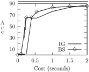
Figure 3(a) plots the accuracy (the percentage of correct identifications) for the policies found for various values of Cmax· In general, the policies produced by BESTSEQ had better accuracy than the ones produced by INFOGAIN. BEST SEQ found different policies for different costs. The bottom 5 rows of Table 1 show how often BESTSEQ used one (resp., two, three, four) operators for different values of Cmax before terminating.
For low cost values (under 0.5 seconds), BESTSEQ per forms much better than INFOGAIN (accuracy of ;:::::65 .33%, versus ;:::::1.78%). As BESTSEQ was able to exploit operator interactions. it was able to apply a second (and probably a third) operator by using a smaller sweep area(£, r) within the allotted time. Since INFOGAIN does not exploit this, it needed significantly more time.
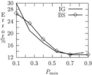
Varying the Minimum Accuracy: In this experiment, we varied Pmin from 0.1 to 0.9. For each of these values, we chose a face randomly from the test set as the target and iden tified it using each of the two policies. During the process, the first person i in the training set for which P( id(h) = i I·) > Pmin is returned (or if cost> Cmax. the most probable face is returned). We repeated this for 30 different faces (runs) per set-up, and repeated the entire process for a total of 15 differ ent set-ups. About 70.4% of these policies matched Figure 2.
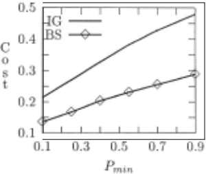
We evaluated the results in two different ways. First, Fig ure 3(b) compares the percentage of wrong identifications of each policy, for each P min value. We see no significant differ ence in error between BESTSEQ and INFOGAIN. The second graph, Figure 3(c), compares the average cost of each policy, for each Pmin value. Here we see that BESTSEQ has much lower cost than IN FOG AIN. Again, this is because BESTS EQ can use operator interactions to sweep a narrower region.
6 Conclusions
Future Work: This paper explored one type of operator in teraction: where theoutputof one operator can be used to help a subsequent operator- here by reducing the time it will re quire to search. Moreover, our operators were relatively sim ple, as they always succeeded (or at least, think that they suc ceed), and they could be run in any order. As a consequence, our policy was quite simple- just straight-line sequence of operators.
There are many ways to extend our analysis. First, it might be useful to allow each operator to return not just a position, but also other information, such as confidence (which would become part of the state). The best policy, then, could use that information when deciding on the proper future action to take. If the abstracted state also included other information about the image, such as average intensity, the policy could use that information as well. This could result in a policy that was more complicated and, presumably, more accurate.
Finally, it would be interesting to consider operators that have some explicit dependency - e.g., one cannot run the "connect edge!" operator unless we have already run some "produce edge!" operator. These precedence constraints would add yet other challenges to our framework.
Contributions: This paper shows how dynamic program ming can be used to build efficient interpretation systems. We argue that computing the utility of operator sequences, which incorporate the benefits of operator interactions, can play a significant role towards building efficient interpretation sys tems. However, in several real world situations, such systems may have (i) to deal with complex and unwieldy states, and (ii) to explore the operator space to find the most promising operator sequence, which is expensive. We addressed the first issue by using simplified abstract states in face recognition, and addressed the second by using an off-line limited looka head search to find the most promising operator sequence.
We framed the image interpretation task as a Markov De cision Problem and used ideas from reinforcement learning to compute the utility of imaging operators non-myopically over a finite lookahead depth in an operator space. We built an in terpretation system that uses these concepts and compared its performance with a successful myopic system in face recog nition. Our results show that the former has a much better per formance in various experiments that address the cost and ac curacy tradeoffs.
(b) Min. Accuracy vs. Error
Acknowledgments
The authors gratefully acknowledges the generous support from Canada's Natural Science and Engineering Research Council and the Alberta Ingenuity Centre for Machine Learn ing.
@inproceedings{ijcai2003p187,
  title     = {Use of Off-line Dynamic Programming for Efficient Image Interpretation},
  author    = {Isukapalli, Ramana and Greiner, Russell},
  booktitle = {Proceedings of the Eighteenth International Joint Conference on
               Artificial Intelligence, {IJCAI-03}},
  publisher = {International Joint Conferences on Artificial Intelligence},
  editor    = {Georg Gottlob and Toby Walsh},
  pages     = {1319--1324},
  year      = {2003},
  url       = {https://ijcai.org/proceedings/2003/187},
}
TY - CPAPER TI - Use of Off-line Dynamic Programming for Efficient Image Interpretation AU - Isukapalli, Ramana AU - Greiner, Russell T2 - Proceedings of the Eighteenth International Joint Conference on Artificial Intelligence, IJCAI-03 PB - International Joint Conferences on Artificial Intelligence PY - 2003 SP - 1319 EP - 1324 UR - https://ijcai.org/proceedings/2003/187 ER -Copied
Machine-readable versions of this paper, for tools and AI agents:





