Thin Junction Tree Filters for Simultaneous Localization and Mapping

1 Introduction

Simultaneous Localization and Mapping (SLAM)-where a robot navigating in an unknown environment must incre­ mentally build a map of its surroundings and localize itself within that map--has attracted significant attention because it is required by many applications in mobile robotics [!hrun, 2002]. Typically the environment is idealized so that 1t con­ sists of an unknown number of stationary "landmarks"; for example, in a given SLAM application these landmarks may be low-level visual features or structural features such as walls and comers. SLAM can then be viewed as the prob­ lem of incrementally estimating the locations of the robot and landmarks from noisy and incomplete observations.

One popular approach treats SLAM as a filtering prob~em [Smith eta/., 1990]. The hidden state of the system at tlme t is represented by a random variable mt which includes. Xt, the state of the robot at time t, and l 1 , ... , ln,, the locatiOns of the nt landmarks observed up to time t. Thus, the size of the state vector is linear in the number of observed landmarks and grows over time. The Kalman filter is used to compute the filtered belief state p( mt I observations to time t), which in this case takes the form of a multivariate Gaussian distribu­ tion N (I-tt, I::t). We regard the mean I-tt as the estimate of the map and the covariance matrix I::t a measure of confidence.

The Kalman filter solution is elegant, but it does not scale well to large SLAM problems. Because I::t explicitly :epre­ sents correlations between all pairs of variables, the stze of the belief state grows as O(nZ); and because each of these correlations must be updated whenever a landmark is re­ observed, the time complexity of its filter operation is also O(nZ). This quadratic complexity renders t~e Ka!man fil­ ter inapplicable to large SLAM problems and gtves nse to the need for principled, efficient approximations.

Unfortunately, the simplest approach--discarding correla­ tions so each variable is estimated independently-presents problems. Ignoring correlations between the robot state and the landmarks' states leads to overconfidence and divergence because correlated observations are treated as if they con­ veyed independent information [Hebert et al., 1996]. Fur­ thermore, correlations between pairs of landmark states are required for quick convergence when the robot closes a loop, i.e., it reobserves known landmarks after an extended pe­ riod of mapping unknown territory (see Figure 1). When the robot closes a loop, it reobserves landmarks whose po­ sitions are known with relative certainty; this helps the robot localize. The robot-landmark correlations translate this im­ proved localization estimate into improved position estimates for recently-observed landmarks. The inter-landmark corre­ lations translate these improved position estimates into im­ provements for the remaining landmarks on the tour. 1 Thus, the correlations give the Kalman filter a valuable property normally associated with smoothing algorithms: it can use current observations to improve estimates "from the past".

Because quadratically many correlations are necessary to close loops, we view the challenge of scalable SLAM filtering as that of estimating and reasoning with quadratically many correlations without quadratic time or space complexity. In this paper, we present a novel and general approximate filter­ ing method satisfying this criterion. Our point of departure

1 Robot-landmark correlations, which decay over time due to mo­ tion noise cannot translate an improved localization estimate into improvem~nts for landmarks observed in the distant past; in con­ trast, inter-landmark correlations do not decay over time.

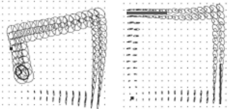
(in Section 2) is to view the filtered belief state of the Kalman filter as a Gaussian graphical model [Cowell eta!., 1999] that evolves over time; this allows us to express correlations in terms of direct dependencies (edges) and indirect dependen­ cies (paths). Analyzing the evolution of this graphical model reveals that filter updates add edges to the graphical model , making inference more expensive. This motivates an approx­ imation scheme in which weak or redundant edges are period­ ically removed to improve the complexity of inference. Note that edge removal is very different than simply discarding cor­ relations; because other edges are left intact, paths-and thus correlations- persist between each pair of variables.

Graphical models give us valuable insight into how good approximate filters can be designed, but using them to rep­ resent the belief state presents problems. First, variable marginals like the robot's current position would not be im­ mediately available as they are in the Kalman filter repre­ sentation; we would require inference to obtain them. Sec­ ond, while it is possible to remove edges from a Gaussian graphical model using the Iterative Proportional Fitting algo­ rithm [Speed and Kiiveri, 1986], its application in this context would be prohibitively slow. Finally, choosing edges whose removal leaves a distribution for which inference is tractable is itself a complicated process [Kja!rulff, 1993].

Our solution to these problems is to use a different rep­ resentation of the belief state. Exact inference in graphical models is often implemented by message passing on a junc­ tion tree [Cowell et a!., 1999]. Rather than view the junction tree algorithm as an "inference engine", we use the junction tree itself as our representation of the belief state. This repre­ sentation has many advantages: the belief state has a "built­ in" inference algorithm (namely, message passing); it gives immediate access to the marginal distribution over any vari­ able; and as we demonstrate, it gives us efficient methods of selecting edges to prune and pruning them.

To implement such a junction tree .filter, we develop meth­ ods for updating the junction tree to reflect filtering updates in Section 3. These updates can cause the width of the junction tree to grow, making inference more expensive; in Section 4 we present a novel "thinning" operation over junction trees called variable contraction. We prove that each variable con­ traction is a maximum likelihood projection that removes a set of edges from the corresponding graphical model. The ap­ proximation error introduced by a variable contraction can be computed efficiently, which allows us to choose which edges to remove at each time step so as to minimize the error.

In Section 5 we apply these techniques to the SLAM prob­ lem and obtain a thin junction tree .filter (TJTF) with a O(nt) space belief state representation and a O(nt ) time filter op­ eration. By delaying the incorporation of recent evidence into the majority of the map, we can improve the filter's time complexity; we present a method of evaluating the signifi­ cance evidence has on different portions of the map, which can be used to adaptively interpolate between constant and linear-time filter operations. Empirically, we find that these adaptive filters choose constant-time updates when mapping new territory, and when closing a loop, they use time lin­ ear in the length of the loop. This is perhaps the best time complexity one would hope for in the SLAM problem, since linearly-many estimates cannot be improved in constant time. Section 6 presents the results of simulation experiments that compare T JTF to other SLAM filters and Section 7 concludes. A companion technical report contains proofs of all proposi­ tions as well as additional background, analysis, and experi­ ments [Paskin, 2002].

1.1 Related work

Significant interest in the SLAM complexity problem has led to a number of approaches [Thrun, 2002]. For example, there are several submap approaches that decompose the prob­ lem into a set of small mapping problems yielding a block­ diagonal landmark covariance matrix. These techniques can achieve constant time complexity, but converge slowly be­ cause information cannot pass between the submaps.

Recently, the FastSLAM algorithm [Montemerlo et a!., 2002]-a Rao-Blackwellized particle filter-has attracted at­ tention because of its logarithmic time complexity. However, our experiments show FastS LAM is susceptible to divergence in large, noisy SLAM problems. We believe this is because the number of particles required for a satisfactory solution can grow exponentially over time; see [Paskin, 2002] for details.

Sparse extended information filters (SElF) [Thrun et a!. , 2002] can be viewed in terms of the graphical model rep­ resentation described above; at each time-step, edges are re­ moved so that a constant-time filter operation can be guaran­ teed. To avoid the additional complexity of inference, SElF employs approximate inference over this approximate model. Thus, the SElF paper provided the valuable insight that sparse graphical models can constitute an efficient solution to SLAM. Implementing this insight while avoiding additional approxi­ mation was one of the primary motivations of this work.

Each of these approaches described above uses a sublinear­ time filter update, and therefore, none can improve all of the landmark estimates in a single update (like the Kalman fil­ ter). T JTF has the best of both worlds: its update step takes constant time unless the observation is significant enough to warrant a linear-time update.

Outside of the SLAM literature, there are two works that are especially relevant. Kjrerulff [ 1993] investigated edge re­ moval as a means of reducing the complexity of inference in graphical models. Our approach is somewhat simpler, as it operates directly on the junction tree without referring to the underlying graphical model. Kjrerulff's analysis of the approximation error inspired ours, and several of his results apply directly to our case.

Thin junction tree filtering is an assumed density filtering (ADF) algorithm because it periodically "projects" the filter's belief state to some tractable family of distributions-in this case, the family of Gaussian distributions characterized by thin junction trees. This makes other work on ADF relevant, especially that of Boyen and Koller [1998], in which the be­ lief state of a dynamic Bayesian network is periodically pro­ jected to a product-of-marginals approximation. In fact, the connection to this work is stronger: Boyen and Koller [1999] extended their earlier analysis to filters where the belief state is represented by a junction tree whose structure evolves over time; however, no algorithms were presented. To our knowl­ edge, T JTF is the first algorithm to which this analysis applies. Here we apply TJTF to a Gaussian graphical model, but noth­ ing prevents its application to the discrete variable networks considered by Boyen and Koller.

2 A graphical model perspective on SLAM

We begin by presenting the SLAM model and then formulat­ ing SLAM filtering in terms of graphical models.

2.1 The SLAM model

We assume a general SLAM model where in each time step the robot moves, obtains an odometry measurement of its motion, and makes several observations of landmarks. As in the Kalman filter context, we assume that the motion and measurement models are known and that they are linear­ Gaussian. 2 The robot motion at time t is governed by

and the odometry measurement Yt at time t is governed by

Yt is typically a noisy measurement of the robot's velocities. Landmark measurements are typically assumed to depend only upon the state of the robot and the state of the observed landmark; for example the observation may consist of the range and bearing to the landmark in the robot's coordinate frame. If the ith landmark measurement at time t issued from landmark j, it is governed by

For simplicity, we assume the correspondence between each measurement and the landmark from which it issued is known. This question of data association, while critically important in SLAM, is largely orthogonal to the issues we address here; in particular, the standard technique of choos­ ing the maximum likelihood data association applies without change in our treatment. When a landmark is first observed, its state variable is added to the belief state with a uninfor­ mative (infinite variance, zero covariance) prior; the measure­ ment update yields an informed posterior estimate of its state.

2 When these models are not linear-Gaussian, they can be approx­ imated as such as in the Extended or Unscented Kalman Filter.

2.2 Gaussian graphical models

Under the assumptions outlined above, the filtered belief state p( mt I Yl:t , Zl:t) is a multivariate Gaussian distribution. The Kalman filter represents this distribution using the moment parameters-the mean vector f.Lt and covariance matrix ~t · If u ""'N(f.L, ~)then its probability distribution is

where d is the length of u. In contrast, Gaussian graphical models are usually based upon the canonical parameters­ the information vector ry and matrix A. If u ""'N 1 ( ry, A)

where a= ~(dlog(27r) IAI + ryT A 1 ry) is the (log) nor­ malization constant. The canonical and moment parameters are related by A= ~ 1 and ry = ~ 1 f.L . An advantage of the canonical parameterization is that multiplication/division of Gaussians reduces to addition/subtraction of the parameters.

Let { ui : i E V} be a set of random variables indexed by elements of the finite set V. We will call a subset of V a family. For a family a <;;;; V, let Ua = { ui : i E a} be the associated set of random variables. A potential over a family a <;;;; V is a non-negative function of Ua. Let F be a set of families and let W = { 1/Ja : a E F} be a set of potential functions over these families. (F, w) defines a distribution

when the normalizer Z = J TiaEF 1/Ja ( ua) du is finite.

The Markov graph associated with (F, w) has vertex set V and a clique of edges over each a E F, i.e., there is an edge between i and j iff ui and u 1 are bound by a potential. The primary value of the Markov graph representation comes from the Hammersley-Clifford theorem, which states that s separates a from b in the Markov graph (for a, b, s <;;;; V) iff Ua JL Ub I U 8 (provided p > 0). In other words, graph separation in the Markov graph encodes the conditional inde­ pendence properties of p. Because conditional independence properties often translate into efficient inference algorithms (e.g., junction tree), the Markov graph gives good intuitions into the design of efficient approximations.

We can represent the Gaussian (5) by a Markov graph, since if we partition the vector u = { u 1 , .. . , un}

where

and Z = e a is the normalization constant. Thus, all the po­ tentials of a Gaussian graphical model are either unary (node potentials) or binary (edge potentials). We also have the im­ portant interpretation that if A ;j = 0, then "1/J{i ,j}(u;,uj) is unity (and therefore superfluous), meaning there is no edge between i and j in the corresponding Markov graph.

2.3 Filtering in Gaussian graphical models

Filtering can be viewed as a three-step procedure: estima­ tion, in which we incorporate the current time step's mea­ surements; prediction, in which we augment the model with the state variables of the next time step; and roll-up, in which we marginalize out the state variables from the past time step. When the measurement and motion models are linear­ Gaussian, the prediction and estimation steps reduce to mul­ tiplying small Gaussian potentials into the model; these up­ dates are summarized by

Proposition 1. 3 Ignoring irrelevant normalization constants, the motion update of equation ( 1) can be implemented by mul­ tiplying the potential

into the model; the odometry measurement update of equation (2) can be implemented by multiplying in the potential

and the landmark measurement update of equation (3) can be implemented by multiplying in the potential

The final step of filtering is roll-up, or marginalizing out the past state. The standard rule for marginalization in the canonical parameterization is given by [Cowell et al., 1999]

then Ua "'N 1 (7]~ 1 , A~) where

The time complexity of computing (11) and (12) is quadratic in the dimension of Ua and cubic in the dimension of u;.

The additive updates above can also be viewed as multiply-. . . IN 1 ( A A 1 1 · mg m a new potentia ai ;; 7];, Aa;A;; A;a) mto the model. The Markov blanket n( i) of i E Vis the set of i's neighbors in the Markov graph. Because missing edges in the Markov graph correspond to zeros in A, we can infer that this is really a potential over n(i), and therefore that marginal­ izing u; out of the model places a clique of edges over the Markov blanket of i.

3 Model parameter indices are omitted for notational simplicity.

2.4 Filtering the SLAM graphical model

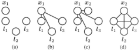
Using these results we can characterize how the structure of the SLAM belief state evolves over time (see Figure 2). For each observed landmark j, we multiply a measurement poten­ tial "1/J(xt , lj) into the graphical model; this adds an edge be­ tween Xt and l j. Thus, after the estimation phase, the robot's state will be connected to the states of all landmarks it has observed. The prediction phase then connects Xt and Xt +1. Finally, the roll-up phase marginalizes out x 1; this places a potential over the Markov blanket of Xt, which now includes all observed landmarks and Xt+l · Now the SLAM graphical model takes the form of a complete graph-i.e., the belief state has no conditional independencies. By induction, this will be true after every time step.

An intuition for why the graphical model becomes dense over time is valuable. When the robot measures a landmark, the landmark's state becomes directly correlated with that of the robot, and thus indirectly correlated with all covariates of the robot state, e.g., other landmark states. When the robot's state is eliminated from the model during roll-up, these indi­ rect correlations must be expressed directly via new edges.

Importantly, these indirect correlations are often much weaker than the direct ones. Thus, even though the SLAM belief state has no true conditional independencies, there are many "approximate" conditional independencies; e.g., the landmarks observed at the beginning and end of a tour are almost independent given those observed in the middle. By removing "weak" edges from the graphical model we can en­ force these approximate conditional independencies so they can be used to speed inference.

3 Junction tree filtering

As discussed in the introduction, the graphical model repre­ sentation is valuable for motivating our approximate filter, but it is not an appropriate representation for its implementation. Instead, we represent the belief state of the filter using a junc­ tion tree. We begin by briefly summarizing the relevant con­ cepts; see [Cowell et al., 1999] for details.

3.1 Junction trees

Let p be a distribution of the form ( 6) with families F and po­ tentials W = { 'l/Ja : a E F}. LetT = ( C, E) be an undirected graph where each vertex (or cluster) c E Cis a subset ofV; T is a junction tree for p if the following three properties hold:

• I . Singly connected property: T is a tree.
• Potential property: For every family a E F there is some cluster c such that c :2 a.
• Running intersection property: Ifi E Vis present in two clusters ci and Cj ofT, it is also present in all clusters on the (unique) path between Ci and Cj.

With each edge { ci, Cj} E E we associate a separator s = ci n Cj; let S be the set ofT's separators.

Given a junction tree T, we can perform inference in the model p by passing messages between the clusters ofT. We begin by associating with T a set of potential functions <P = { ¢c : c E C} U { ¢s : s E S}, one for each cluster and separator. The charge on T is defined to be

We initialize <P by setting all cluster and separator potentials to unity, multiplying each potential 'ljJ E W into ¢c for some c E C (which is possible by the potential property), and mul­ tiplying z-I into an arbitrary ¢c; then ¢r = p.

Let c and d be adjacent clusters with separator s = c n d. Passing a message from c to d updates the separator potential ¢s and the cluster potential ¢d as follows:

Importantly, these updates leave the charge (13) invariant, so ¢r = p. Thus, we can view them as reparameterizing the distribution p. When messages are passed along every edge in both directions (in an appropriate schedule), the cluster and separator potentials are updated so that they are marginals of p over their respective variables. A junction tree in this state is called consistent and it can be used to obtain marginals over any set of variables that reside together in some cluster.

When T has no nonmaximal clusters, ICI ::; lVI so the number of messages required for inference is bounded by 2 · IV 1- In the case of a Gaussian graphical model, the cluster and separator potentials are Gaussians; if they are represented by their canonical parameters, the time complexity of passing a message is dominated by the cost of the marginalization in (14) which is implemented via (11) and (12); thus, it is at worst cubic in the size of the cluster. In sum, inference is linear in lVI and cubic in the width ofT, traditionally defined as the size of the largest cluster minus one.

3.2 Incremental junction tree maintenance

We adopt consistent junction trees as the belief state represen­ tation of our filter; i.e., the belief state will be represented by the charge (13) of a consistent junction tree. Recall from Sec­ tion 2.3 that the prediction and estimation phases of the filter update can be implemented by multiplying in small, simple potentials to the probability distribution, and that the roll­ up phase is implemented by marginalizing variables out of the model. In this section we describe how to incrementally maintain a consistent junction tree under these updates.

In what follows we will make use of three nonstandard op­ erations to restructure a consistent junction tree.

• Cloning: To clone a cluster c, we create a copy d, attach d to c with separators = c = d, and set¢; = ¢'d = ¢c·
• Merging: Let c and d be neighboring clusters with sep­ arators. To merged into c, we: (1) update c* = cUd; (2) update ¢~ = ¢c¢d/¢s; (3) swing all edges incident to dover to c; and (4) removed from C and s from S.
• Pushing: Let c and d be neighboring clusters with sep­ arator s such that i E c but i tf. d. To push i from c to d we update s* = s U {i} and d* = d U {i} and pass a message from c to d to update ¢s and ¢d· By extension we can push i from c to a nonadjacent clus­ ter d by successive pushes along the unique path from c to d. (Any nonmaximal clusters created by pushing are subsequently merged into their subsuming neighbors.)

It is easy to check that all of these operations preserve the three structural constraints as well as the charge and consis­ tency of a junction tree.

Multiplying in potentials

Assume our belief state is represented by a consistent junc­ tion tree T. In order to update the charge ofT to reflect the multiplication of a potential 'l/Ja ( ua) into p, we must find a cluster c :2 a and multiply 'l/Ja into ¢c· To restore consistency, we could pass messages throughout T, but this is twice the work needed: a simple consequence of the message-passing updates (14) and (15) is that we need only distribute evidence from c, i.e, we must pass messages along edges in a preorder traversal from c.

If there is no cluster that covers the family a of the new po­ tential, then we must first modify the junction tree T to create one. Draper [ 1995] presents several techniques to do this; in the Gaussian case the problem is somewhat simpler, since the potentials bind at most two variables. When multiplying in an edge potential 1/J( u;, Uj) requires us to create a cluster cover­ ing {i,j}, we find the closest pair of clusters c and d such that i E c and j E d and push i from c to d. We then multiply 1/J( ui, Uj) into ¢d( ud) and distribute evidence from d.

It is worth noting that in several cases, conditional inde­ pendencies obviate the evidence distribution step. This is a significant optimization, since message passing is by far the most expensive operation. This occurs, for example, when performing the prediction step (because Xt+l is an unob­ served directed leaf of the graphical model and therefore does not impact the distributions of the other nodes), when ob­ serving a landmark for the first time (due to its uninformative prior), and in certain types of odometry updates.

Marginalizing out variables

Assume again that we have a consistent junction tree T rep­ resenting p. As described in Section 2.3, marginalizing u; out of p places a potential over the Markov blanket of ui. Be­ cause the junction tree must have a cluster that covers this new potential, marginalizing out ui is not as simple as marginal­ izing it out of all the cluster potentials that bind it.

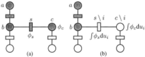
Let n(i) be the Markov blanket of i. Because T has the potential property, we are guaranteed that n(i) ~ UcEC,c3 ic, i.e., that i's Markov blanket is covered by the clusters con­ taining i. (In fact, in the sequel this containment will often be strict equality.) Moreover, because T has the running inter­ section property, all clusters containing i constitute a subtree ofT, which we denote Ti . By successively merging the clus­ ters of Ti into each other, we can obtain a new junction tree where i resides in a single cluster c* ;-;? n( i). Marginalizing ui out of this junction tree is simple: we remove i from c* and marginalize Ui out of c/Jc·. It is simple to check that this operation results in a consistent junction tree for J p( u) dui.

4 Thinning the junction tree

The updates described in the previous section can cause the clusters of the junction tree to grow; in particular, the merging of clusters required by marginalizations can cause the width of the junction tree to increase quickly. The complexity of message passing scales with the width of the junction tree, and therefore our goal is to define a "thinning" operation that reduces the width (see Figure 3):

Definition 1. Let i E V appear in more than one cluster of the consistent junction tree T, let c be a leaf of Ti (the subtree ofT induced by i), and let s be the separator joining c to Ti . A variable contraction of i from c removes i from c and s and marginalizes ui out of c/Jc and cp3 · (cis merged into its subsuming neighbor if it becomes nonmaximal.)

We now consider some properties of variable contraction.

Proposition 2. Variable contractions preserve consistency and the singly connected and running intersection properties. Thus, the new junction tree is valid for some distribution, although perhaps not p: the potential property may be vio­ lated. Variable contraction is local and efficient: it requires marginalizing a variable out of one cluster potential and one separator potential, which in the Gaussian case can be accom­ plished in O(lcl 2 ) time using (11) and (12). Also, variable contraction is a general method of"thinning" a junction tree:

Proposition 3. In combination with cloning, variable con­ traction can reduce the width of any junction tree.

The following proposition relates the original distribution and the distribution resulting from a variable contraction:

Proposition 4. Let T be the junction tree obtained from the variable contraction of Definition 1. Then c/Jt minimizes the Kullback-Liebler divergence D( c/Jr II ·) over all distributions in which Ui JL Uc- s I Us\ i·

Alternatively, the probability distribution represented by T has maximum likelihood (under the original junction tree's distribution) over all distributions in which u i is conditionally independent of Uc-s given us\i· Thus, we can consider each variable contraction to be a maximum likelihood projection that cuts edges between i and c- s.

To reduce the width of a given junction tree, we should choose the variable contraction that minimizes the approxi­ mation error, which we take to be the Kullback-Liebler di­ vergence from the original to the approximate distribution, D( c/Jr II c/Jt ). This approximation error can be computed effi­ ciently, as shown by the following result ( cf. [Kja:rulff, 1993, Theorem 11]):

Proposition 5. Let T be the junction tree obtained from the variable contraction of Definition 1. Then

To compute the conditional mutual information (16) we need only the marginal p( uc). In a consistent junction tree, this marginal is simply c/Jc, and therefore the approximation er­ ror of a variable contraction can be computed locally. When p( uc) is a Gaussian distribution, the computation is espe­ cially efficient: its cost depends only the dimension of u i.

Proposition 6. Let c index a set of Gaussian random vari­ ables Uc, let s ~ c, and let i E s. Then

Ac and A" are parameters of the potentials c/Jc and ¢., so we can simply extract from each the sub-blocks corresponding to ui and compute the difference of their log determinants.

5 Thin junction tree filters for SLAM

We have now assembled most of the machinery required to design a thin junction tree filter for the SLAM problem. All that remains is the logic to decide into which clusters new po­ tentials are multiplied and also how variable contractions are employed to thin the junction tree. There are many possibil­ ities; the method below presents a nice compromise between simplicity and performance. We then describe a refinement that can reduce the time complexity from linear to constant.

5.1 Linear-time approximate filtering

Recall from Section 3.1 that if the width of our junction tree is k, then it will require O(IVIk 2 ) space and message pass­ ing will take O(IVIk 3 ) time. In SLAM [VI = nt + 1, so we can obtain a O(nt) space filter with a O(nt) time filter opera­ tion by periodically thinning the junction tree so that its width remains bounded by a constant k.

We start with roll-up. When the robot state Xt is marginal­ ized out, we must merge all of the clusters in which it resides. In the worst case Xt can reside in all of the clusters, in which case our belief state will collapse to one large cluster. To pre­ vent this, we iteratively contract Xt (choosing the contraction that minimizes the error (17) each time) until it resides in only one cluster c. Then, we perform the time update, which con­ sists of multiplying the motion potential 'l/;(xt, Xt+l) into c/Jc. marginalizing Xt out of c, multiplying the odometry potential 'l/;(xt+d into c/Jc, and distributing evidence from c.

When multiplying in a landmark measurement potential 'l/;(xt,l j ) for a landmark that is currently in the model, we use the method of Section 3.2, i.e., we push Xt until it resides in a cluster c with l1. (This may increase the sizes of some clusters, but the subsequent contraction of Xt in the next roll­ up ensures this increase in cluster size is temporary.) We then multiply 'l/;( Xt , l j) into cPc and distribute evidence from c.

If instead the landmark j has not previously been observed, we must add the new variable l 1 to the model. If the smallest cluster that contains Xt (call it c) can admit another variable without violating the width limit k, we add l 1 to c and multi­ ply 'l/;(xt, lj) into cPc· If not, then we clone c to obtain d, con­ tract Xt until it resides only in d, and thin d via a sequence of greedy optimal variable contractions. A cluster overlap parameter h governs the size to which dis thinned, and there­ fore how many variables reside in the separator s that joins it to c (since in this case s = d \ Xt). If h is small, d will admit more new landmark variables before another cloning is required; the trade-off is that its separator s will shrink, reducing the amount of information it can transmit.

5.2 Constant-time approximate filtering

The linear time complexity of the filter above arises mainly because we pass messages to every cluster each time we dis­ tribute evidence from some cluster c. We can get a constant­ time filter operation by employing a lazy message passing scheme, where we distribute evidence only to constantly many nearby clusters; the approximation is that the marginals of the remaining clusters will not be conditioned on the obser­ vation. This introduces minimal error when the observation is uninformative about distant variables; this occurs, e.g., when the robot is mapping new territory. Moreover, because we are still updating the charge correctly, this approximation is temporary: at any later time a full round of message passing (taking linear time) will yield the same estimate we would have obtained by passing all messages at every time step.

Alternatively, we can interpolate between the linear-time update and this constant-time update by employing an adap­ tive message passing scheme in which messages are propa­ gated only as long as they induce significant changes in the belief state. If we define "significant" sensibly, this scheme will take constant time when mapping new territory; when closing loops, it will take time linear in the length of the loop.

We measure the significance of a message ci --7 c1 over the separators by D(¢: II cPs). the Kullback-Liebler diver­ gence from the new separator marginal to the original separa­ tor marginal. In the Gaussian case this is

where cPs = N(p,, E) and ¢; = N(p,* , E*). Importantly, the significance of evidence propagated from a cluster ci to another cluster ck (measured in this way) decreases with the distance between them in the junction tree [Kjrerulff, 1993, Theorem 13]. Thus, if a message was not significant for a cluster, it need not continue the evidence distribution.

6 Experiments

Here we present a summary of our findings ; the technical re­ port contains more detail and further experiments.

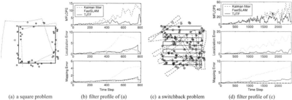
We compared TJTF, the Kalman filter, and FastSLAM on large-scale SLAM simulations in which a robot moves around in a square world that is populated with uniformly distributed point-landmarks. Its motion and measurement models are all subject to significant noise and are linearized using the un­ scented transformation. We used two types of trajectories: a square loop (similar to that a robot mapping an indoor en­ vironment might travel) and a switchback trajectory (which could be used to map a large open area). Noise and controls were determined in advance so the robot followed the desired path and each filter received identical observations.

Figure 4 shows two examples of our simulations. The filters are evaluated by their computational cost (millions of floating point operations), localization error (the distance from the robot's position to the filter's estimate) and map er­ ror (the average distance from each landmark to the filter's estimate). TJTF was run with the width limit k = 16, the cluster overlap h = 4, and adaptive message passing with the significance threshold set at 0.1 nats; FastS LAM was run with 100 particles, as recommended in [Montemerlo et al., 2002].

We found that the estimation error of TJTF with maxi­ mum cluster sizes as small as 16 can be comparable with the Kalman filter, and that it gets smaller as k increases. This indicates that the edges removed by T JTF indeed carry little information; it also suggests that the estimation error of TJTF will be at least competitive with that of SElF (an approximate form of the Kalman filter) and less than that of the submap approaches (which neglect long-distance correlations).

We also found that TJTF is good at closing loops; in Figure 4(b) we can see the localization and mapping error of T JTF suddenly drop at t = 780, when the robot first reobserves its starting point; also evident is a sudden increase in the compu­ tational cost: the filter is choosing to update the entire map in linear time rather than using cheaper constant-time updates. We found that FastSLAM had difficulty closing large loops (notice its divergence in Figure 4(b)) and that its estimation error in general was larger than that of TJTF.

Finally, using accurate counts of floating point operations, we found that TJTF can be as fast as FastSLAM, and that it becomes more efficient than the Kalman filter when the map contains a few hundred or more landmarks.

7 Conclusion

We believe thin junction tree filters are a promising ap­ proximation technique for dynamic probabilistic inference. First, they are flexible, in that they allow the practitioner to trade computational complexity for approximation accuracy by varying the width of the junction tree and the depth of evidence propagation. Second, the error of each local ap­ proximation can be computed exactly, giving an important indication of how trustworthy the approximate estimates are. Finally, the T JTF approximation is context sensitive in that it is not chosen in advance; rather, the approximation is chosen adaptively to minimize the approximation error.

When applied to the SLAM problem, TJTF performs com­ petitively with the exact filter, but with superior asymptotic space and time complexity. Interestingly, the approach pre­ sented here has significant connections to both the submap approach and SElF. First, like SElF, TJTF cuts "weak" edges from the graphical model to speed inference; however, in T JTF we can use exact inference over this approximate model, whereas SElF must use approximate inference. Second, the belief state of a T JTF has a natural interpretation as a coupled set of local maps, just as in the submap approaches. In par­ ticular, each cluster of the junction tree can be viewed as a submap. The T JTF formulation gives concrete semantics to the relationships between the maps, including how they must be updated, how consistency is maintained, and how the set of local maps can be determined online to minimize the ap­ proximation error subject to a complexity constraint.

Acknowledgements

I gratefully acknowledge Intel Corporation for supporting this research via an Intel Research Internship, as well as Bar­ bara Engelhardt, Kevin Murphy, Stuart Russell, and Sekhar Tatikonda for valuable comments on a draft of this paper.