
A New Method For The Three Dimensional Container Packing Problem
Proceedings of the Seventeenth International Joint Conference on Artificial Intelligence. Pages 342-349.
© 2001 International Joint Conferences on Artificial Intelligence
Abstract
A new algorithm for solving the three dimensional container packing problem is proposed in this paper. This new algorithm deviates from the traditional approach of wall building and layering. It uses the concept of “building growing” from multiple sides of the container. We tested our method using all 760 test cases from the OR-Library. Experimental results indicate that the new algorithm is able to achieve an average packing utilization of more than 87%. This is better than the results reported in the literature.
- [B.K. and K., 1993] Ngoi B.K. and Whybrew K. A fast spa- tial representation method. Journal of International Ad- vance Manufacturing Technology, 8(2), 1993.
- [E.E. and M.D., 1990] Bischoff E.E. and Marriott M.D. A comparative evaluation of heuristics for container loading. European Journal of Operational Research, 44:267-276, 1990.
- [E.E and Ratcliff, 1995] Bischoff E.E and MSW Ratcliff. Is- sues in the development of approaches to container load- ing. Omega. Int. J. Mgmt Sci., 23(4):337-390, 1995.
- [Gehring H. and M., 1990] Menschner K. Gehring H. and Meryer M. A compute-based heuristic for packing pooled shipment containers. European Journal of Operational Research, 1(44):277-288, 1990.
- [Han C.P. and J.P., 1989] Knott K. Han C.P. and Egbelu J.P. A heuristic approach to the three-dimensional cargo- loading problem. Int. J. Prod. Res., 27(5):757-774, 1989.
- [J.A and B.F., 1980] George J.A and Robinson B.F. A heuristic for packing boxes into a container. Computer and Operational Research, 7:147-156, 1980.
- [K.A. and W.B., 1992] Dowsland K.A. and Dowsland W.B. Packing Problems. European Journal of Operational Re- search, 56:2-14, 1992.
- OR-Lib, ] OR-Lib. http://www.ms.ic.ac.uk/library/. Link
- [T.H. and Nee, 1992] Loh. T.H. and A.Y.C. Nee. A pack- ing algorithm for hexahedral boxes. In Proceedings of the Conference of Industrial Automation, Singapore, pages 115-126, 1992.
- [Wang, 2001] Ying Wang. 3D container packing. Honours thesis, National University of Singapore, 2001.
- [W.B., 1991] Dowsland W.B. Three dimensional packing- solution approaches and heuristic development. Interna- tional Journal of Operational Research, 29:1637-1685, 1991.
References were extracted automatically from the PDF and may contain errors.
Full text extracted automatically from the PDF; figures, tables and equations may differ. The PDF is the version of record.
1 Introduction
Packing boxes into containers is a common problem faced by the logistics and transportation industries. The three dimensional (3D) packing problem is a difficult extension of the two dimensional (2D) stock cutting problem and the one dimensional (1D) bin packing problem. Even the 1D bin packing problem is known to be NP-Complete. For a survey of packing problems, please refer to [K.A. and W.B., 1992]. While pseudo-polynomial time algorithms have been derived for the 1D packing problem, no such results have been derived for the 3D packing problem.
The 3D packing problem can be divided into two main variants. The first variant is: given a list of boxes of various sizes, pack a subset of these boxes into one container to maximize the volume utilization of the container. The second variant is: given a list of boxes of various sizes, pack all the boxes into as few containers as possible. In addition, constraints, such as orientation restriction, weight distribution, locality restriction, may be imposed on the boxes.
In this paper, we study the packing problem that maximizes the volume utility of a single container with orientation restrictions on the boxes.
Many different heuristics have been developed to "optimize" volume utilization in a single container. [J.A and B.F., 1980] proposed a primitive "wall-building" method. [Gehring H. and M., 1990] proposed an improved "wallbuilding" heuristic. [T.H. and Nee, 1992] proposed a layering approach. [Han C.P. and J.P., 1989] provided an algorithm for packing identical boxes, which is a combination of "wallbuilding" and layering. [B.K. and K., 1993] proposed a data structure for representing the boxes and free spaces, which is used in their heuristic. [E.E. and M.D., 1990] presented a comparative evaluation of different heuristic rules for freight container loading with the objective of minimizing the container length needed to accommodate a given cargo. [W.B., 1991] examined a number of heuristic rules for the problem. The emphasis on both wall building and layering is to create walls or layers of boxes as flat as possible. At all times, the methods attempt to retain a flat forward packing face. The existing methods most mirror the hand-packing process, which is a natural way to solve the problem. However, they put many restrictions on the location of the boxes which may not be feasible to the actual application. Another problem of the existing approaches is that they may leave a thin layer of nonuseful empty spaces near the entrance or the ceiling of the container, which results in space underutilization. Also, the papers in the existing literature used data that are not easily accessible, hence, it is relatively hard to compare the various methods quantitatively.
In this paper, we propose a new method. Boxes are packed into container in "building-growing" fashion instead of "wall building" manner. Furthermore, each wall of the container can be treated as base to locate the boxes, which provides more flexibility. We tested our program on all the 760 test cases in [OR-Lib, ]. Our experimental results indicate that we are able to achieve an average packing utilization more than 87%.
2 Problem Specification
We are given a set of rectangular boxes a0 ✁ ✄ ✆ ✞ ✠ ☛ ☛ ☛ ✠ ✆ ✍ ✏ and a rectangular container ✒ . Let ✓ ✔ , ✖ ✔ and ✘ ✔ represent the three dimensions of the box ✆ ✔ , and ✙ , ✚ , and ✛ represent the three dimensions of the container.
The objective of the problem is to select a subset ✜ ✢ a0 and assign a position to each box, ✆ ✤ ✥ ✜ , in the 3D space of container ✒ such that ✧ ★ ✪ ✬ ✮ ✓ ✤ ✱ ✖ ✤ ✱ ✘ ✤ is maximized subjected to the constraints that all boxes must be totally contained in ✒ , no two boxes intersect in 3D space and every edge of the packed box must be parallel or orthogonal to the container walls.
3 Multi-Directional Building-Growing Algo
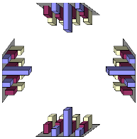
The idea of this 3D packing algorithm [Wang, 2001] comes from the process of constructing a building. When erecting a building, we construct the basement on the ground first, then the building will "rise up" floor by floor. Here, the box will play the role of the floor, and the wall of the container will act as the ground. Boxes are placed on the wall of the container first as it builds the basement on the ground. After which, other boxes will be placed on top of the basement boxes. Following this process, boxes will be placed one on top of another, just like the construction of a new building. Every wall of the container can be treated as the ground for boxes to stack on. However, the users reserve the right to choose the walls to act as the ground. Note that, this algorithm does not take into consideration whether packed boxes form a flat layer or not, which is the main idea of the "wall building" approach. Figure 1 illustrates the main idea of this algorithm.
3.1 Formulation of the Algorithm
Overall Packing Process
After getting the option from the user for the acting-asground walls, this algorithm reads in the container and box information, including length, width, height, orientation and quality information, from the data file. The algorithm then orders the boxes according to certain criteria. Subsequently, actual packing will be performed based on the best matching between base area of boxes and empty spaces. The following pseudo code presents the overall algorithm.
main a0 1. get wall option() 2. read in the container information (length,width,height) 3. for(every box of type b) a0 1.read in b's information(length,width,height,orientation,quantity) 2.bn=create box nodes(box b) 3.insert box node(box node bn) ✁ 4. pack() ✁get wall option()
Users are free to choose which of the walls of a container to be used as ground/base. Basically, all the empty spaces created from one ground(wall) form an empty space list. There are at most six empty space lists as shown in Figure 2.
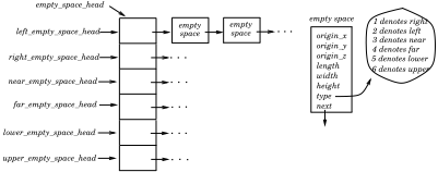
An empty space in each empty space list has its own origin and coordinate system as shown in Figure 3. Here the lower coordinate system is the "normal" coordinate system.
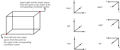
The initial value of each empty space list head is the whole container. If the user does not choose wall ✂ as the ground, then empty space list ✂ 's head should be pointing to null. Note that each empty space list ✂ only takes care of all the empty spaces using wall ✂ as base, without knowing the existence of the other empty space lists. Because of the exact and accurate representation, empty spaces may overlap with each other.
create box nodes(box b)
Every box has three attributes namely, length, width and height. Length is measured along the x-axis, so is width along the y-axis and height along the z-axis. And the area surrounded by length and width is called the base area of a box. There is a unique id assigned to each box, yet, there are six orientations associated with it (see Figure 4. Note that a number is used to denote each edge of the box.).
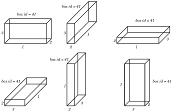
For each type of box (same type of box means boxes with same length, width and height), at most six box nodes will be created for them but with the same id. Each box node represents a possible orientation for one type of box. If a certain orientation is not allowed, this algorithm will simply omit the box node of that orientation.
| box1 | box2 | box3 | box4 | box5 | box6 | |
|---|---|---|---|---|---|---|
| id | 41 | 41 | 41 | 41 | 41 | 41 |
| length | 1 | 2 | 1 | 3 | 2 | 3 |
| width | 2 | 1 | 3 | 1 | 3 | 2 |
| height | 3 | 3 | 2 | 2 | 1 | 1 |
insert box node(box node bn)
Whenever a box information is obtained from the data file, a new box node will be created and inserted to the box node list based on the function below. Given a newly created box node ✆ a0 ✁ , this algorithm goes through the box node list, and for each existing box node ✆ a0 ✞ , calculates the priority number for ✆ a0 ✞ and ✆ a0 ✁ respectively as follows:
✄ ☎ ✝ ✟ ☎ ✝ ☛ ✌ ✍ ✏ ✑ ✓ ✕ ✗ ✙ ✟ ✜ ✄ ✢ ☎ ✥ ✙ ✟ ✜ ✧ ✩ ✑ ✍ ✏ ✑ ✓ ✕ ✙ ✟ ✜ ✧ ✩ ✑ ✍ ✏ ✑ ✬ ✕ ✯ ✱ ✝ ✩ ✄ ✢ ☎ ✥ ✏ ✝ ✵ ✍ ✏ ✑ ✓ ✕ ✏ ✝ ✵ ✍ ✏ ✑ ✬ ✕ ✄ ☎ ✝ ✟ ☎ ✝ ☛ ✌ ✍ ✏ ✑ ✬ ✕ ✗ ✙ ✟ ✜ ✄ ✢ ☎ ✥ ✙ ✟ ✜ ✧ ✩ ✑ ✍ ✏ ✑ ✬ ✕ ✙ ✟ ✜ ✧ ✩ ✑ ✍ ✏ ✑ ✓ ✕ ✯ ✱ ✝ ✩ ✄ ✢ ☎ ✥ ✏ ✝ ✵ ✍ ✏ ✑ ✬ ✕ ✏ ✝ ✵ ✍ ✏ ✑ ✓ ✕where parameters vol per and dim per denote the volume priority percentage and the biggest dimension priority percentage respectively; routines ✸ ✹ ✺ ✼ ✽ ✿ ❁ ✆ a0 ❂ and ✆ ✂ ❃ ❁ ✆ a0 ❂ return the volume and the biggest dimension of box ✆ inside box node bn respectively. After getting ❄ ❅ ✂ ✹ ❅ ✂ ❈ ✖ ❁ ✆ a0 ✞ ❂ and ❄ ❅ ✂ ✹ ❅ ✂ ❈ ✖ ❁ ✆ a0 ✁ ❂ , the algorithm compares these two numbers:
- ❍ if ❄ ❅ ✂ ✹ ❅ ✂ ❈ ✖ ❁ ✆ a0 ✁ ❂ ■ ❄ ❅ ✂ ✹ ❅ ✂ ❈ ✖ ❁ ✆ a0 ✞ ❂ , insert ✆ a0 ✁ to the front of ✆ a0 ✞ .
- ❍ otherwise, continue to compare ❄ ❅ ✂ ✹ ❅ ✂ ❈ ✖ ❁ ✆ a0 ✁ ❂ with the priority number of the box node behind ✆ a0 ✞ .
According to the above, a box node nearer to the head possesses either larger volume or one bigger dimension, hence, has higher priority to be packed into the container first. Note that boxes with the same id but with different orientations are located adjacent to each other, and they have the same priority to be packed into the container, because they are actually the same box.
pack()
In every attempt to pack one box into the container, the algorithm finds a most suitable empty space for each of the first ✂ box nodes with the sane priority number,in terms of the percentage of the base area of that box occupies the base area of the empty space. Inside all these ✂ pairs of box node and empty space, the algorithm finds one pair ( ✆ a0 ✠ ✹ ✿ ) with the greatest base area occupation percentage ❄ ,
- ❍ remove ✆ a0 , if ❄ ■ ▲ .
- ❍ pack ✆ a0 , if ❄ ◆ ❖ a80 ✂ a0 ❃ ❄ ✿ ❅ ◗ ❄ ◗ ▲ .
- ❍ decide to pack or remove ✆ a0 carefully, if ❚ ❯ ❄ ❯ ❄ ◆ ❖ a80 ✂ a0 ❃ ❄ ✿ ❅
The following pseudo code illustrates the packing process of the algorithm.
while(box node head!=null) a0 for(box node ✏ ✑ ❨ with same priority as box node head) a0 for(every empty space oe in the 6 empty space lists) a0 percentage( ✏ ✑ ❨ )= ❩ ❬ ❭ ❪ ❬ ❫ ❪ ❬ ❴ ❩ ❛ ❜ ❝ ❩ ❬ ❭ ❪ ❬ ❫ ❪ ❬ ❴ ❞ ❪ ❝ ✁ ✁ find one pair (bn,oe) with greatest p=percentage(bn) if( ✄ ❢ ❤ ) a0 //bn cannot be packed into any empty space remove ✏ ✑ //because ✏ ✑ is too big to be packed into any empty space now //and empty space will become smaller and smaller, there will //be no chance for bn to be packed into any empty space later ✁ if( ✄ ❥ ❦ ❧ ✝ ✑ ✵ ✄ ✢ ☎ ♥ ✄ ♥ ❤ ) a0 1.create a packed box ✄ ✏ according to oe's coordinate system, then convert it to the normal coordinate system and insert it into packed box list 2.delete one box id from box node ✏ ✑ 3.update empty space(empty space oe,packed box pb) ✁ if(0 a115 ✄ a115 packing per) a0 //in this case, we cannot find a good fit between ✏ ✑ and oe, //so we need to decide whether we can drop the first ✝ box //nodes with the same priority number if(after removing the first ✝ box nodes and ✧ a116 ❞ ✈ ✇ ① ❪ ❴ ③ ⑤ ❪ ❫ ❪ ❭ ③ ✇ ❛ ⑥ ❬ ⑦ ⑧ ❪ ⑨ ❩ ❞ ⑩ ❪ ❭ ❶ ③ ⑤ ❪ ⑥ ❬ ⑦ ⑧ ❪ ⑨ ❩ ❞ ⑩ ❪ ❭ ❝ a116 ❞ ✈ ✇ ① ❪ ❴ ⑦ ❞ ❛ ③ ❬ ❨ ❛ ❪ ❫ ❝ ❹ moving per) a0 remove the first ✝ box nodes //because without these few difficult-to-be-packed box nodes, //we may still get good utilization ✁ else a0 1.create a packed box ✄ ✏ according to oe's coordinate system then convert it to the normal cooridnate system and insert it into packed box list 2.delete one box id from box node ✏ ✑ 3.update empty space(empty space oe,packed box pb) ✁ ✁ ✁update empty space(empty space oe,packed box pb)
After a box is packed into the container, the original set of empty spaces will be modified by the newly packed box ❄ ✆ . Moreover, ❄ ✆ will not only affect the empty space ✹ ✿ it resides in, but also the empty spaces nearby ✹ ✿ , because, in order to represent the empty spaces effectively, the empty spaces overlap. The responsibility of this routine is to update the empty spaces after one box is placed into the container. This process can be performed using the following two steps:
Step 1: Change ❄ ✆ to the coordinate system which ✹ ✿ lies in and absorb the new empty spaces out of ✹ ✿ (Figure 5).
Updating ✹ ✿ :
- Remove ✹ ✿ from its empty space list
- If ( ✿ ❺ ✞ ✠ ✿ ❺ ✁ ✠ ✿ ❺ ❻ are not inside the empty space list ✹ ✿ resides in)
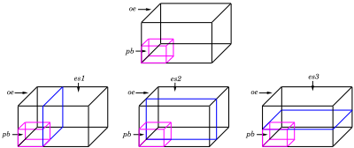
insert it(them) into the empty space list ✹ ✿ resides in
Step 2: For every empty space ✿ in the six empty space lists,
- Convert ❄ ✆ to the coordinate systemwhich ✿ is in
- Test whether there is overlap between ✿ and ❄ ✆ , and update ✿ accordingly
All the possible overlap cases between ✿ and ❄ ✆ will be disscussed below and the update method will be given by the end. case 1: pb intersects one corner of e.
e.g. pb intersects the lower left near corner of e.
case 2: pb intersects one entire edge of e.
e.g. pb intersects the left edge of upper plane of e.
case 3: pb intersects the inner part of one edge of e.
e.g. pb intersects part of lower left edge of e.
case 4: pb gets into e from one plane of it without touching any corner point of e.
e.g. pb gets into e from the left plane of e.
case 5: pb cuts away one entire plane of e.
e.g. pb cuts away the whole left plane of e.
case 6: pb crosses one pair of parallel edges of e without touching any corner point of e
- e.g. pb crosses the upper horizontal pair of edges of e.
case 7: pb passes through one pair of parallel planes of e without touching any corner point of e
e.g. pb passes through the near-far planes of e.
case 8: pb cuts e into two new empty space.
- e.g. pb cuts e into two new empty space from vertical direction.
case 9: the whole pb resides inside e.
case 10: pb covers the whole e.
Updating ✿ in each case above:
- Remove ✿ from its empty space list
- If (newly created empty spaces ✿ ❺ empty space list ✿ resides in)
- are not inside the
- insert it(them) into the empty space list ✿ resides in
3.2 Experimental Results
This algorithm was successfully implemented using the Java Programming Language. All the experiments were run on an Alpha 600MHz machine running the Digital Unix operating system. The OR-Library [OR-Lib, ] has a collection of test data for a variety of OR problems. There are nine sets of test data with 760 test cases for the 3D packing problem. All the test data in [OR-Lib, ] have been tested.
The algorithm was tuned using various parameter settings. The packing result for test file 8 is omitted in all result presentations, because of the fact that we can pack every box into the container in most cases and the size of the container is much larger than the total size of the boxes to be packed into the container.
The best packing result in terms of container volume utilization is shown in Figure 6. The parameter and wall combination used for the best packing result is shown in Table 2.
| Parameter packing vol=0.95 moving per=1.0 vol per=0.9 dim per=0.1 | Wall Combination left wall right wall far wall lower wall |
In the experimental results shown in Figure 6, the X-axis represents the test case index and the Y-axis represents the container volume utilization.
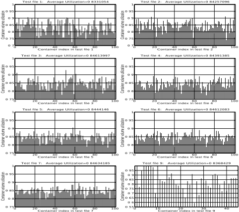
Using this parameter setting and wall combination, the average container volume utilization for all the available test cases in the OR-Library (except dest file 8) can reach as high as 0.84285194. This utilization is comparable to the published result of the existing literature. Moreover, the special advantage of this algorithm is its speed as it needs about two seconds to pack one container.
On the other hand, the container volume utilization can still be improved for the price of efficiency. In the next section, an improvement phase is introduced.
4 Incorporating a Look-AheadMechanism
In the packing process of Multi-Directional BuildingGrowing (MDBG) approach, the algorithm only chooses one pair of best fit box and empty space in terms of base area occupation percentage among the most difficult-to-be-packed boxes. MDBG Algorithm only takes care of the local information, and the decision made by this algorithm doesn't contain any knowledge for the future. The look-ahead mechanism not only considers the current pairing, but also looks at its potential effect.
4.1 Look-Ahead Improvement Strategy
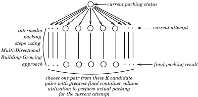
The strategy will choose a80 pairs of boxes and empty spaces with the greatest base area occupation percentage. Each one of these a80 pairs of boxes and empty spaces will be assumed to be the chosen pair for this attempt and be temporarily packed into the container, and the packing process is continued using the MDBG approach from this attempt onwards until all the boxes have been packed into the container or no more boxes can be packed into it. Then based on the final container volume utilization, the improvement strategy will choose one pair of the box and empty space from the initial a80 pairs, which gives best final container volume utilization. This chosen pair of box and empty space will then be used as the actual packing for this attempt. This pair of box and empty space satisfies both best fit currently and best potential effect in the future. Figure 7 illustrates the look-ahead idea.
The following is the pseudo-code for the look-ahead improvement strategy.
newpack() a0 while(there's box in the box node list) a0 //attempt to pack one box into the container //1.get K boxes with greatest base area occupation percentage for(every box b in the box node list) a0 for(every empty space in the 6 empty space lists) a0 find a best fit empty space e for b with greatest base area occupation percentage p ✁ if( ✄ ❢ ❤ ) a0 //b cannot be packed into any empty space remove b ✁ else if(top K base area occupation percentages a115 p ♥ 1) a0 replace e and b into the top K best fit pairs✁ ✁ //2. using MDBG approach pack the K candidate pairs for(i=1..k) a0 1.temporarily pack ✏ ❨ to empty space ✢ ❨ at this attempt 2.continue packing using pack() in section 3 3.record down the final container volume utilization at ✧ ❨ ✁ //3.get one box with the greatest final utilization from the K // candidates, and use this box in the actual packing of this // attempt find one box b from ✏ ❨ and one empty space ✢ from ✢ ❨ with greatest final container volume utilization ✧ pack b into e permanently ✁ ✁4.2 Experimental Results
In the last section, using MDBG approach, we have experimented with all the test data using all possible wall combinations for many possible parameter settings. The best packing result comes from the wall combination: left wall, right wall, far wall, lower wall; and the parameter setting: ❄ ◆ ❖ a80 ✂ a0 ❃ ✸ ✹ ✺ ✁ ❚ ☛ a0 ✁ ✠ ✽ ✹ ✸ ✂ a0 ❃ ❄ ✿ ❅ ✁ ▲ ☛ ❚ ✠ ✸ ✹ ✺ ❄ ✿ ❅ ✁ ❚ ☛ a0 ✠ ✄ ✂ ✽ ❄ ✿ ❅ ✁ ❚ ☛ ▲ . Based on this experience, the LookAhead mechanism is tested on all data files using this parameter setting and wall combination, and let a80 go from 1 to 6. The results are summarized in the tables below:
| k=1 | k=2 | k=3 | k=4 | k=5 | k=6 | |
|---|---|---|---|---|---|---|
| file1 | 0.81054 | 0.83601 | 0.85984 | 0.86713 | 0.87859 | 0.88356 |
| file2 | 0.81704 | 0.83970 | 0.86335 | 0.86457 | 0.87433 | 0.87576 |
| file3 | 0.82474 | 0.83616 | 0.85437 | 0.86468 | 0.86952 | 0.87036 |
| file4 | 0.83225 | 0.84148 | 0.85376 | 0.85925 | 0.87081 | 0.87068 |
| file5 | 0.83525 | 0.84282 | 0.85540 | 0.86260 | 0.86822 | 0.87072 |
| file6 | 0.83403 | 0.84009 | 0.85665 | 0.86275 | 0.86534 | 0.86679 |
| file7 | 0.83761 | 0.84349 | 0.85048 | 0.86072 | 0.86260 | 0.86575 |
| file9 | 0.84885 | 0.87370 | 0.88711 | 0.89616 | 0.90393 | 0.90656 |
| average | 0.82862 | 0.84196 | 0.85809 | 0.86505 | 0.87193 | 0.87399 |
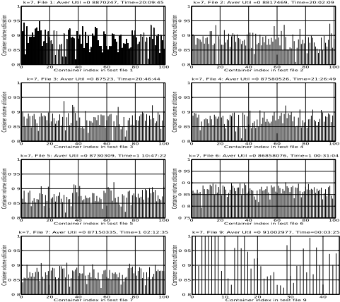
For the look-ahead method,the best packing result comes from the wall combination: left wall, right wall, far wall, upper wall and the parameter setting: ❄ ◆ ❖ a80 ✂ a0 ❃ ✸ ✹ ✺ ✁ ❚ ☛ a0 ✁ ✠ ✽ ✹ ✸ ✂ a0 ❃ ❄ ✿ ❅ ✁ ▲ ☛ ❚ ✠ ✸ ✹ ✺ ❄ ✿ ❅ ✁ ❚ ☛ a0 ✠ ✄ ✂ ✽ ❄ ✿ ❅ ✁ ❚ ☛ ▲ . The average container volume utilization using this best parameter setting and wall combination can be increased to 0.87813642. The detailed packing result is listed in Figure 8.
Note that in the experimental results shown in Figure 8, the X-axis represents the test case index and the Y-axis represents the container volume utilization, and the average packing utilization and packing time are indicated on the top of each figure.
5 Comparison of Results
To show the effectiveness of the proposed packing algorithm and its coupled improvement strategy, we compare our results run on the test problems from the [OR-Lib, ] with results in [E.E and Ratcliff, 1995] which is the only available work in the existing literature containing packing results on 700 test problems from the OR-Library.
| scheme(a) | scheme(b) | scheme(c) | MDBGAlgo | LAM | |
|---|---|---|---|---|---|
| file1 | 81.76% | 83.79% | 85.40% | 83.31% | 88.70% |
| file2 | 81.70% | 84.44% | 86.25% | 84.26% | 88.17% |
| file3 | 82.98% | 83.94% | 85.86% | 84.61% | 87.52% |
| file4 | 82.60% | 83.71% | 85.08% | 84.39% | 87.58% |
| file5 | 82.76% | 83.80% | 85.21% | 84.44% | 87.30% |
| file6 | 81.50% | 82.44% | 83.84% | 84.61% | 86.86% |
| file7 | 80.51% | 82.01% | 82.95% | 84.63% | 87.15% |
In Table 4, the scheme(a), scheme(b), scheme(c) are the respective scheme a, b and c in [E.E and Ratcliff, 1995]. MDBG Algo refers to the Multi-Directional BuildingGrowing Algorithm, and LAM refers to Look-Ahead Mechanism. From the experiment results, it is clear that the container volume utilization using the MDBG Algorithm is slightly better than that of scheme a and b in [E.E and Ratcliff, 1995]. But the MDBG Algorithm coupled with the LAM produces a much higher container volume utilization than scheme c in [E.E and Ratcliff, 1995]. The experimental results provide a strong evidence that the Multi-Directional Building-Growing Algorithm when coupled with the LookAhead mechanism gives an significant improvement to the container volume utilization for 3D container packing problem.
6 Conclusion
In this paper, we presented a new approach to solving the 3D container packing problem. Our paper is the first paper to benchmark our results across all the OR-Benchmarks. Our packing utilization of 87% compares very favorably against past works in this area.
@inproceedings{ijcai2001p49,
  title     = {A New Method For The Three Dimensional Container Packing Problem},
  author    = {Lim, Andrew and Ying, Wang},
  booktitle = {Proceedings of the Seventeenth International Joint Conference on
               Artificial Intelligence, {IJCAI-01}},
  publisher = {International Joint Conferences on Artificial Intelligence},
  editor    = {Bernhard Nebel},
  pages     = {342--349},
  year      = {2001},
  url       = {https://ijcai.org/proceedings/2001/49},
}
TY - CPAPER TI - A New Method For The Three Dimensional Container Packing Problem AU - Lim, Andrew AU - Ying, Wang T2 - Proceedings of the Seventeenth International Joint Conference on Artificial Intelligence, IJCAI-01 PB - International Joint Conferences on Artificial Intelligence PY - 2001 SP - 342 EP - 349 UR - https://ijcai.org/proceedings/2001/49 ER -Copied
Machine-readable versions of this paper, for tools and AI agents:





