
A Hybrid Approach for the 01 Multidimensional Knapsack problem
Proceedings of the Seventeenth International Joint Conference on Artificial Intelligence. Pages 328-332.
© 2001 International Joint Conferences on Artificial Intelligence
Abstract
We present a hybrid approach for the 0–1 multidimensional knapsack problem. The proposed approach combines linear programming and Tabu Search. The resulting algorithm improves significantly on the best known results of a set of more than 150 benchmark instances.
- [Aboudi and Jörnsten, 1994] R. Aboudi and K. Jörnsten. Tabu Search for General Zero-One Integer Programs us- ing the Pivot and Complement Heuristic. ORSA Journal of Computing, 6(1):82-93, 1994.
- [Balas and Martin, 1980] E. Balas and C.H. Martin. Pivot and a Complement Heuristic for 0-1 Programming. Man- agement Science, 26:86-96, 1980.
- [Chu and Beasley, 1998] P.C. Chu and J.E. Beasley. A ge- netic algorithm for the multidimensional knapsack prob- lem. Journal of Heuristic, 4:63-86, 1998.
- [Dammeyer and Voß, 1993] F. Dammeyer and S. Voß. Dy- namic tabu list management using the reverse elimination method. Annals of Operations Research, 41:31-46, 1993.
- [Drexl, 1988] A. Drexl. A simulated annealing approach to the multiconstraint zero-one knapsack problem. Comput- ing, 40:1-8, 1988.
- [Fréville and Plateau, 1993] A. Fréville and G. Plateau. Sac à dos multidimensionnel en variable 0-1 : encadrement de la somme des variables à l'optimum. Recherche Opérationnelle, 27(2):169-187, 1993.
- [Gavish and Pirkul, 1982] B. Gavish and H. Pirkul. Allo- cation of data bases and processors in a distributed com- putting system. Management of Distributed Data Process- ing, 31:215-231, 1982.
- [Gavish and Pirkul, 1985] B. Gavish and H. Pirkul. Efficient algorithms for solving multiconstraint zero-one knapsack problems to optimality. Mathematical Programming, 31:78-105, 1985.
- [Glover and Kochenberger, 1996] F. Glover and G.A. Kochenberger. Critical event tabu search for multidi- mensional knapsack problems. In I.H. Osman J.P. Kelly, editor, Metaheuristics: The Theory and Applications, pages 407-427. Kluwer Academic Publishers, 1996.
- [Glover and Laguna, 1997] F. Glover and M. Laguna. Tabu Search. Kluwer Academic Publishers, 1997.
- [Glover, 1990] F. Glover. Tabu search. ORSA Journal of Computing, 2:4-32, 1990.
- [Hanafi and Fréville, 1998] S. Hanafi and A. Fréville. An ef- ficient tabu search approach for the 0-1 multidimensional knapsack problem. European Journal of Operational Re- search, 106:659-675, 1998.
- [Osorio et al., 2000] M.A. Osorio, F. Glover, and Peter Ham- mer. Cutting and surrogate constraint analysis for im- proved multidimensional knapsack solutions. Techni- cal report, Hearin Center for Enterprise Science. Report HCES-08-00, 2000.
- [Shih, 1979] W. Shih. A branch & bound method for the multiconstraint zero-one knapsack problem. Journal of the Operational Research Society, 30:369-378, 1979.
- [Toyoda, 1975] Y. Toyoda. A simplified algorithm for ob- taining approximate solutions to zero-one programming problem. Management Science, 21(12):1417-1427, 1975.
References were extracted automatically from the PDF and may contain errors.
Full text extracted automatically from the PDF; figures, tables and equations may differ. The PDF is the version of record.
1 Introduction
The NP-hard 0-1 multidimensional knapsack problem (MKP01) consists in selecting a subset of a0 given objects (or items) in such a way that the total profit of the selected objects is maximized while a set of knapsack constraints are satisfied. More formally, the MKP01 can be stated as follows.
where ✂ ☛ IN ✘ ✗ , ✝ ☛ IN ✙ ✚ ✗ and ✠ ☛ IN ✙ . The binary components ✆ ✢ of ✆ are decision variables: ✆ ✢ ✣ ✓ if the object ✦ is selected, ✎ otherwise. ✂ ✢ is the profit associated to ✦ . Each of the ★ constraints ✝ ✩ ✄ ✆ ✞ ✠ ✩ is called a knapsack constraint.
The special case of theMKP01 with ★ ✣ ✓ is the classical knapsack problem (KP01), whose usual statement is the following. Given a knapsack of capacity ✠ and a0 objects, each being associated a profit (gain) and a volume occupation, one wants to select ✯ (✯ ✞ a0 and ✯ not fixed) objects such that the total profit is maximized and the capacity of the knapsack is not exceeded. It is well known that the KP01 is not strongly NP-hard because there are polynomial approximation algorithms to solve it. This is not the case for the general MKP01.
The MKP01 can formulate many practical problems such as capital budgeting where project ✦ has profit ✂ ✢ and consume ✲ ✳ ✩ ✢ ✵ units of resource ✶ . The goal is to determine a subset of the a0 projects such that the total profit is maximized and all resource constraints are satisfied. Other important applications include cargo loading [Shih, 1979], cutting stock problems, and processor allocation in distributed systems [Gavish and Pirkul, 1982]. Notice that the MKP01 can be considered as a general 0-1 integer programming problem with non-negative coefficients.
Given the practical and theoretical importance of the MKP01, it is not surprising to find a large number of studies in the literature; we give a brief review of these studies in the next section.
2 State of the Art
Like for many NP-hard combinatorial optimization problems, both exact and heuristic algorithms have been developed for the MKP01. Existing exact algorithms are essentially based on the branch and bound method [Shih, 1979]. These algorithms are different one from another according to the way the upper bounds are obtained. For instance, in [Shih, 1979], Shih solves, exactly, each of the ★ single constrained, relaxed knapsack problems and select the minimum of the ★ objective function values as the upper bound. Better algorithms have been proposed by using tighter upper bounds, obtained with other MKP01 relaxation techniques such as lagrangean, surrogate and composite relaxations [Gavish and Pirkul, 1985]. Due to their exponential time complexity, exact algorithms are limited to small size instances ( a0 ✣ ✷ ✎ ✎ and ★ ✣ ✹ ).
Heuristic algorithms are designed to produce near-optimal solutions for larger problem instances. The first heuristic approach for the MKP01 concerns for a large part greedy methods. These algorithms construct a solution by adding, according to a greedy criterion, one object each time into a current solution without constraint violation. The second heuristic approach is based on linear programming by solving various relaxations of the MKP01. A first possibility is to relaxe the integrality constraints and solve optimally the relaxed problem with simplex. Other possibilities include surrogate and composite relaxations [Osorio et al., 2000].
More recently, several algorithms based on metaheuristics have been developed, including simulated annealing [Drexl, 1988], tabu search [Glover and Kochenberger, 1996; Hanafi and Fr´eville, 1998] and genetic algorithms [Chu and Beasley, 1998]. The metaheuristic approach has allowed to obtain very competitive results on large instances compared with other methods ( a0 ✣ ✹ ✎ ✎ and ★ ✣ ✻ ✎ ).
Most of the above heuristics use the so-called pseudoutility criterion for selecting the objects to be added into a solution. For the single constraint case (the KP01), this criterion corresponds to the profit/resource ratio. For the general MKP01, the pseudo-utility is usually defined as ✂ ✢ ✼ ✲ ✾ ✄ ✳ ✢ ✵
where ✾ is a multiplier for the column vector ✆ ✢ . Notice that it is impossible to obtain "optimal" multipliers. Thus the pseudo-utility criterion may mislead the search.
In this paper, we propose an alternative way to explore the search space. We use fractional optimal solutions given by linear programming to guide a neighborhood search (Tabu Search or TS) algorithm. The main idea is to exploit around a fractional optimal solution with additional constraints. We experiment this approach on a very large variety of MKP01 benchmark instances and compare our results with the best known ones. We show that this hybrid approach outperforms previously best algorithms for the set of tested instances.
The paper is organized as follows. Next section presents the general scope of our approach. Section 4 describes the algorithm used to determine promising sub-space of the whole search space from where we run a TS algorithm. This algorithm is presented in section 5. Finally we give computational results on a large set of MKP01 instances in section 6.
3 AHybrid Approach for the MKP01
The basic idea of our approach is to search around the fractional optimum a0 ✆ of some relaxed MKP. Our hypothesis is that the search space around a0 ✆ should contain high quality solutions 1 .
This general principle can be put into practice via a two phase approach. The first phase consists in solving exactly a relaxation MKP of the initial MKP01 to find a fractional optimal solution a0 ✆ . The second phase consists in exploring carefully and efficiently some areas around this fractional optimal point.
Clearly, there are many possible ways to implement this general approach. For this work, we have done the following choices. The first phase is carried out by using simplex to solve a relaxed MKP. The second phase is ensured by a Tabu Search algorithm.
Let us notice first that relaxing the integrality constraints alone may not be sufficient since its optimal solution may be far away from an optimal binary solution. To be convinced, let us consider the following small example with five objects and one knapsack constraint:
This relaxed problem leads to the fractional optimal solution a0 ✆ ✣ ✲ ✓ ✑ ✓ ✑ ✌ ✎ ✏ ✑ ✎ ✑ ✎ ✵ with an optimal cost value a0 ✒ ✣ ✻ ✎ ✄ ✻ while the optimal binary solution is ✆ ✓ ✕ ✗ ✣ ✲ ✎ ✑ ✎ ✑ ✓ ✑ ✓ ✑ ✓ ✵ with an optimal cost value ✒ ✓ ✕ ✗ ✣ ✷ ✹ .
However, the above relaxation can be enforced to give more precise information regarding the discrete aspect of the problem. To do this, let us notice that all solutions of MKP01 verify the property: ✙ ✗ ✢ ✚ ✎ ✆ ✢ ✣ ✯ ☛ IN with ✯ an integer. Now if we add this constraint to the relaxed MKP, we obtain a series of problems:
1 This hypothesis is confirmed by experimental results presented later. Of course, the hypothesis does not exclude the possibility that other areas may contain good solutions.
where ✥ ✲ ✆ ✵ is the sum of the components of ✆ , defining a hyperplane. We have thus several (promising) points a0 ✆ ✦ ★ ✩ around which a careful search will be carried out.
To show the interest of this extra constraint, take again the previous example with ✯ ✣ ✓ ✑ ✷ ✑ ✻ , leading to three relaxed problems:
MKP[ ✓ ] ✪ a0 ✒ ✦ ✎ ✩ ✣ ✓ ✷ et a0 ✆ ✦ ✎ ✩ ✣ ✲ ✓ ✑ ✎ ✑ ✎ ✑ ✎ ✑ ✎ ✵ MKP[✷ ] ✪ a0 ✒ ✦ ✬ ✩ ✣ ✷ ✮ et a0 ✆ ✦ ✬ ✩ ✣ ✲ ✓ ✑ ✓ ✑ ✎ ✑ ✎ ✑ ✎ ✵ MKP[✻ ] ✪ a0 ✒ ✦ ✯ ✩ ✣ ✷ ✹ et a0 ✆ ✦ ✯ ✩ ✣ ✲ ✎ ✑ ✎ ✑ ✓ ✑ ✓ ✑ ✓ ✵where ✯ ✣ ✻ gives directly an optimal binary solution ✆ ✦ ✯ ✩ ✣ ✆ ✓ ✕ ✗ without further search.
In general cases, search is necessary to explore around each fractional optimum and this is carried out by an effective TS algorithm (Section 5). In order not to go far away from each fractional optimum a0 ✆ ✦ ★ ✩ , we constraint TS to explore only the points ✆ ☛ ✱ such that ✳ ✆ ✑ a0 ✆ ✦ ★ ✩ ✳ , the distance between ✆ and a0 ✆ ✦ ★ ✩ is no greater than a given threshold ✵ ✙ ✶ ✸ 2 .
To sum up, the proposed approach is composed of three steps:
- determine interesting hyperplanes ✥ ✲ ✆ ✵ ✣ ✯ ;
- run simplex to obtain the corresponding fractional optimum a0 ✆ ✦ ★ ✩ ;
- run Tabu Search around each a0 ✆ ✦ ★ ✩ , limited to a sphere of fixed radius.
4 Determine Hyperplanes ✺ ✻ ✽ ✾ ❀ ❁ and Simplex Phase
Given an a0 size instance ofMKP01, it is obvious that the a0 ❃ ✓ values ✎ ✞ ✯ ✞ a0 do not have the same interest regarding the optimum. Furthermore exploring all the hyperplanes ✥ ✲ ✆ ✵ ✣ ✯ would be too much time consuming. We propose, in this section, a simple way to compute good values of ✯ .
Starting from a 0-1 lower bound ✒ (i.e. a feasible solution obtained by a previous heuristic), the method consists in solving, with the simplex algorithm, the two following problems:
Let ✥ ★ ✶ a0 be the optimal value of this problem. A knapsack that holds fewer items than ✯ ✙ ✩ ✗ ✣ ❉ ✥ ★ ✶ a0 ❋ respects no longer the constraint ✂ ✄ ✆ ❆ ✲ ✒ ❃ ✓ ✵ .
Let ✥ ★ ✳ ✆ be the optimal value of this problem. It is not possible to hold more items than ✯ ✙ ✶ ✸ ✣ ❍ ✥ ★ ✳ ✆ ❏ without violate one of the ★ constraints ✝ ✩ ✄ ✆ ✞ ✠ ✩ .
2 This point is discussed more formally in section 5.2.
Consequently, local search will run only in the hyperplanes ✥ ✲ ✆ ✵ ✣ ✯ for which ✯ is bounded by ✯ ✙ ✩ ✗ and ✯ ✙ ✶ ✸ . Hence we compute, using once again the simplex algorithm, the ✲ ✯ ✙ ✶ ✸ a0 ✯ ✙ ✩ ✗ ❃ ✓ ✵ relaxed MKP ✢ ✯ ✤ which give us the continuous optima a0 ✆ ✦ ★ ✩ which are used by the TS phase.
5 Tabu Search Phase
A comprehensive introduction of Tabu Search may be found in [Glover and Laguna, 1997]. We give briefly below some notations necessary for the understanding of our TS algorithm ✁ ✂ ☎ ✝ ✟ .
5.1 Notations
The following notations are specifically oriented to the MKP01:
- ✡ a configuration ✆ is a binary vector with a0 components;
- ✡ the unconstrained search space ✱ is defined to equal the set ✌ ✎ ✑ ✓ ✕ ✗ , including both feasible and unfeasible configurations;
- ✡ a move consists in changing a small set of components of ✆ giving ✆ ☛ and is denoted by ★ ✌ ✎ ✲ ✆ ✑ ✆ ☛ ✵ ;
- ✡ in this binary context, the flipped variables of a move can be identified by their indexes in the ✆ vector: These indexes are the attributes of the move;
- ✡ the neighborhood of ✆ , ✒ ✲ ✆ ✵ , is the subset of configurations reachable from ✆ in one move. In this binary context, a move from ✆ to ✆ ☛ ☛ ✒ can be identified without ambiguity by the attribute ✦ if ✆ ☛ is obtained by flipping the ✦ ✗ ✔ element of ✆ . More generally, we use ★ ✌ ✎ ✲ ✶ ✎ ✑ ✶ ✬ ✑ ✄ ✄ ✄ ✑ ✶ ★ ✵ to denote the move ★ ✌ ✎ ✲ ✆ ✑ ✆ ☛ ✵ where ✖ ✦ ☛ ✢ ✓ ✑ ✯ ✤ ✆ ☛ ✩ ✗ ✣ ✓ a0 ✆ ✩ ✗ . Such a move is called a ✯ ✂ ✘ ✳ a0 ✚ ✛ .
5.2 Search Space Reduction
Regarding the knapsack constraints ( ✝ ✄ ✆ ✞ ✠ ), ✱ ✣ ✌ ✎ ✑ ✓ ✕ ✗ is the completely relaxed search space. It is also the largest possible search space. We specify in this section a reduced search space ✢ ✣ ✱ which will be explored by our Tabu Search algorithm. To define this reduced space, we take the ideas discussed previously (Section 3):
- limitation of ✱ to a sphere of fixed radius around the point a0 ✆ ✦ ★ ✩ , the optimal solution of the relaxed MKP ✢ ✯ ✤ . That is: ✳ ✆ ✑ a0 ✆ ✦ ★ ✩ ✳ ✞ ✵ ✙ ✶ ✸ ;
- limitation of the number of objects taken in the configurations ✆ , that are visited by the tabu search algorithm, to the constant ✯ (intersection of ✱ and the hyperplane ✥ ✲ ✆ ✵ ✣ ✯ ).
For the first point, we use ✙ ✗ ✢ ✚ ✎ ✳ ✆ ✢ a0 ✆ ☛ ✢ ✳ to define the distance ✳ ✆ ✑ ✆ ☛ ✳ where ✆ et ✆ ☛ may be binary or continuous. We use the following heuristic to estimate the maximal distance ✵ ✙ ✶ ✸ authorized from the starting point a0 ✆ ✦ ★ ✩ . Let ✲ ✓ ✑ ✓ ✑ ✥ ✥ ✥ ✑ ✓ ✑ ✦ ✎ ✑ ✥ ✥ ✥ ✑ ✦ ★ ✑ ✎ ✑ ✥ ✥ ✥ ✑ ✎ ✵ be the elements of the vector a0 ✆ ✦ ★ ✩ sorted in decreasing order. ✦ ✢ are fractional components of a0 ✆ ✦ ★ ✩ and we have: ✓ ✪ ✦ ✎ ❆ ✦ ✬ ❆ ✥ ✥ ✥ ❆ ✦ ★ ✪ ✎ . Let u be the number of the components having the value of
1 in a0 ✆ ✦ ★ ✩ . In the worst case, we select ✦ ✢ items rather than the ✾ components. With ✥ ✲ a0 ✆ ✦ ★ ✩ ✵ ✣ ✯ that gives ✵ ✦ ★ ✩ ✣ ✷ ✯ ✲ ✾ ❃ ✱ a0 ✯ ✵ . If ✾ ✣ ✯ , it follows ✵ ✦ ★ ✩ ✣ ✎ that corresponds to the case where a0 ✆ ✦ ★ ✩ is a binary vector. Depending on the MKP01 instances, we choose ✵ ✙ ✶ ✸ ☛ ✢ ✎ ✄ ✲ ✯ ✵ ✦ ★ ✩ ✑ ✷ ✯ ✵ ✦ ★ ✩ ✤ . Hence, each tabu process running around a0 ✆ ✦ ★ ✩ has its own search space ✢ ★ :
Note that all ✢ ★ are disjoint, this is a good feature for a distributed implementation of our approach.
Finally, in order to further limit TS to interesting areas of ✢ ★ , we add a qualitative constraint on visited configurations:
where ✒ ✙ ✩ ✗ is the best value of a feasible configuration found so far.
5.3 Neighborhood
Aneighborhoodwhich satisfies the constraint ✥ ✲ ✆ ✵ ✣ ✯ is the classical add/drop neighborhood: we remove an object from the current configuration and add another object to it at the same time. This neighborhood is used in this study. The set of neighboring configurations ✒ ✲ ✆ ✵ of a configuration ✆ is thus defined by the formula:
It is easy to see that this neighborhood is a special ase of ✷ ✂ ✘ ✳ a0 ✚ ✛ (cf. sect. 5.1). We use in the following sections indifferently ★ ✌ ✎ ✲ ✆ ✑ ✆ ☛ ✵ or ★ ✌ ✎ ✲ ✶ ✑ ✦ ✵ with ✆ ☛ ✩ ✣ ✓ a0 ✆ ✩ and ✆ ☛ ✢ ✣ ✓ a0 ✆ ✢ . As TS evaluates the whole neighborhood for a move, we have a time complexity of ✸ ✲ ✲ a0 a0 ✯ ✵ ✯ ✯ ✵ for each iteration of ✁ ✂ ☎ ✟ ✝ .
5.4 Tabu List Management
The reverse elimination method (✻ ✼ ✾ ), introduced by Fred Glover [Glover, 1990], leads to an exact tabu status (i.e. ★ ✌ ✎ ✲ ✆ ✑ ✆ ☛ ✵ tabu ❀ ✆ ☛ has been visited). It consists in storing in a running list the attributes (pair of components) of all completed moves. Telling if a move is forbidden or not needs to trace back the running list. Doing so, one builds another list, the so-called residual cancellation sequence (✻ ❁ ✂ ) in which attributes are either added, if they are not yet in the ✻ ❁ ✂ , or dropped otherwise. The condition ✻ ❁ ✂ ✣ ❃ corresponds to a move leading to a yet visited configuration. For more details on this method see [Dammeyer and Voß, 1993; Glover, 1990]. ✻ ✼ ✾ has a time complexity ✸ ✲ ✶ ✎ ✛ ✦ ✬ ✵ (✶ ✎ ✛ ✦ is the current value of the move counter).
For our specific ✷ ✂ ✘ ✳ a0 ✚ ✛ move, we need only one trace of the running list. Each time we meet ✳ ✻ ❁ ✂ ✳ ✣ ✷ , the move with ✻ ❁ ✂ ✏ and ✻ ❁ ✂ ✎ attributes is said tabu. Let ✶ ✎ ✛ ✦ be the move counter. The following algorithm updates the tabu status of the whole neighborhood of a configuration ✆ and corresponds to the equivalence
Algorithm 1: UPDATE TABU ✩ a0 ✁ ✄ ✆ % end of running list repeat ✩ a0 ✩ ✞ ✎ ✢ a0 running list ✦ ✩ ✩ if ✢ ✟ ✡ ☞ ✍ then ✡ ☞ ✍ a0 ✡ ☞ ✍ ✏ ✢ else ✡ ☞ ✍ a0 ✡ ☞ ✍ ✒ ✢ if ✓ ✡ ☞ ✍ ✓ ✚ ✬ then ✗ ✶ ✔ ✕ ✦ ✡ ☞ ✍ ✗ ✩ ✦ ✡ ☞ ✍ ✙ ✩ a0 ✩ ✗ ✁ ✄ ✗ ✶ ✔ ✕ ✦ ✡ ☞ ✍ ✙ ✩ ✦ ✡ ☞ ✍ ✗ ✩ a0 ✩ ✗ ✁ ✄ until ✩ ✚ ✏This algorithm traces back the running list table from its ✛ ✦ ✛ a0 ✓ entry to its ✎ entry.
5.5 Evaluation Function
We use a two components evaluation function to assess the configurations ✆ ☛ ✂ : ✜ ✔ ✲ ✆ ✵ ✣ ✙ ✩ ✓ ✶ ✢ ✸ ✤ ✔ ✢ ✲ ✳ ✩ ✄ ✆ a0 ✠ ✩ ✵ and ✒ ✲ ✆ ✵ ✣ ✂ ✄ ✆ . To make a move from ✆ , we take among ✆ ☛ ☛ ✒ ✲ ✆ ✵ the configuration ✆ ☛ defined by the following relation:
Random choice is used to break ties.
Each time ✜ ✔ ✲ ✆ ✵ ✣ ✎ the running list is reset and ✒ ✙ ✩ ✗ is updated. Hence the tabu algorithm explores areas of the search space where ✒ ✪ ✒ ✙ ✩ ✗ trying to reach feasibility.
5.6 Tabu Algorithm
Based on the above considerations, our TS algorithm for MKP01 ( ✁ ✂ ☎ ✟ ✝ ) works on a series of problems like:
where ✒ ✙ ✩ ✗ is a strictly increasing sequence. Let ✳ ✻ ✄ ✩ ✄ ✳ be the running list size. Considering the last feature of our algorithm given just above (sect. 5.5), ✳ ✻ ✄ ✩ ✄ ✳ is twice the maximum number of iterations without improvement of the cost function. The starting configuration ✆ ✩ ✗ ✩ ✗ is built with the following simple greedy heuristic: Choose the ✯ items ✌ ✶ ✎ ✑ ✥ ✥ ✥ ✑ ✶ ★ ✕ , which have the largest a0 ✆ ✦ ★ ✩ ✩ ✗ value.
6 Computational Results
All the procedures of ✁ ✂ ☎ ✟ ✝ have been coded in C language. Our algorithm has been executed on different kind of CPU (up to 20 distributed computers like PII350, PIII500, ULTRASPARC5 and 30). For all the instances solved below, we run ✁ ✂ ☎ ✟ ✝ with 10 random seeds (0..9) of the standard srand() C function.
We have first tested our approach on the 56 classical problems used in [Aboudi and J¨ornsten, 1994; Balas and Martin, 1980; Chu and Beasley, 1998; Dammeyer and Voß, 1993; Drexl, 1988; Fr´eville and Plateau, 1993; Glover and Kochenberger, 1996; Shih, 1979; Toyoda, 1975]. The size of these problems varies from a0 =6 to 105 items and from ★ =2 to 30 constraints. These instances are easy to solve for state-of-theart algorithms. Indeed, our approach finds the optimal value
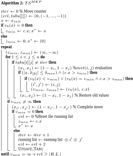
(known for all these instances) in an average time of 1 second (details are thus omitted). The running list size ( ✳ ✻ ✄ ✩ ✄ ✳ ) is fixed to 4000.
For the next two sets of problems, the running list size ( ✳ ✻ ✄ ✩ ✄ ✳ ) is fixed to 100000. Hence the maximum number of moves without improvement is 50000.
The second set of tested instances is constituted of the last seven (also the largest ones with a0 ✣ 100 to 500 items, ★ ✣ 15 to 25 constraints) of 24 benchmarks proposed by Glover and Kochenberger [Glover and Kochenberger, 1996]. These instances are known to be particularly difficult to solve for Branch & Bound algorithms. Table 1 shows a comparison between our results (columns 4 to 7) and the best known ones reported in [Hanafi and Fr´eville, 1998] (column ✁ ❯ ❱ ).
| GK | ✗ ✚ ✙ | ✪ ❲ ❳ | ✽ ❀ | ★ ❀ | ✩ ✗ ✁ ✄ ❀ | ❨ ✁ ✿ ✴ ❀ | ✦ ★ ✩ |
|---|---|---|---|---|---|---|---|
| ✎ ❩ | ✎ ✏ ✏ ✚ ✬ ❬ | ❪ ❬ ✬ ❪ | ❴ ❵ ❛ ❜ | ❝ ✎ | ✯ ❝ ❩ ✯ | ✎ ✏ | ❬ ❩ ✴ ✴ ❝ ❪ |
| ✎ ❞ | ✎ ✏ ✏ ✚ ✬ ❬ | ✯ ❩ ❝ ❝ | ❡ ❜ ❢ ❣ | ❬ ✎ | ✯ ✎ ❪ ❪ | ❞ | ❪ ❞ ✴ ✴ ❬ ❬ |
| ✬ ✏ | ✎ ✏ ✏ ✚ ✬ ❬ | ❬ ✎ ✌ ✌ | ❵ ❤ ❜ ❥ | ✌ ✏ | ✬ ✏ ❩ ✏ | ❬ | ❝ ✎ ✴ ✴ ✌ ❪ |
| ✬ ✎ | ✎ ✏ ✏ ✚ ✬ ❬ | ✯ ✎ ❞ ❬ | ❡ ❛ ❥ ❥ | ❪ ✬ | ✎ ❪ ❝ ❬ | ❪ | ❪ ✏ ✴ ✴ ❪ ❝ |
| ✬ ✬ | ✎ ✏ ✏ ✚ ✬ ❬ | ✬ ❬ ✬ ✎ | ❛ ❵ ❛ ❡ | ✯ ❪ | ❬ ✎ ✬ | ✬ | ✯ ✎ ✴ ✴ ✯ ✌ |
| ✬ ✯ | ✬ ✏ ✏ ✚ ✎ ❬ | ❞ ✬ ✯ ✎ | ❣ ❛ ❡ ❵ | ✎ ✬ ✯ | ✎ ❝ ❞ ✌ ❝ | ✎ ✯ ✎ | ✎ ✎ ❞ ✴ ✴ ✎ ✬ ❝ |
| ✬ ❪ | ❬ ✏ ✏ ✚ ✬ ❬ | ❞ ✏ ❝ ✬ | ❣ ❥ ❦ ❥ | ✎ ✎ ❞ | ❞ ✬ ✎ ✏ | ✬ ❝ ❩ | ✎ ✎ ❝ ✴ ✴ ✎ ✬ ❬ |
Column ✯ ✘ shows the number of items of the best solution ✆ ✘ with cost ✒ ✘ found by ✁ ✂ ☎ ✝ ✟ . From the table, we observe that all the results are improved. Columns ✶ ✎ ✛ ✦ ✘ and ❧ ✛ ✂ ✄ ✘ give the number of moves and the time elapsed to reach ✆ ✘ . We know that the algorithm runs 50000 moves after ✶ ✎ ✛ ✦ ✘ . The search process takes thus an average of 380 seconds for the test problems GK18...GK22, 600 seconds for GK23 and 1100 seconds for GK24. Last column gives the ✯ hyperplane's values visited by ✁ ✂ ☎ ✝ ✟ .
The third set of test problems concerns the 30 largest benchmarks ( a0 ✣ ✹ ✎ ✎ items, ★ ✣ ✻ ✎ constraints) of ORLibrary 3 , proposed recently by Chu and Beasley [Chu and Beasley, 1998].
| CB | a0 ✁ ✄ ✆ | ✽ ❀ | ★ ❀ | ✩ ✗ ✁ ✄ ❀ | ❨ ✁ ✿ ✴ ❀ | ✦ ★ ✩ |
|---|---|---|---|---|---|---|
| ✯ ✏ ✴ ❬ ✏ ✏ ✴ ✏ | ✎ ✎ ❬ ❩ ❝ ❩ | ❤ ❤ ❵ ❣ ❵ ❥ | ✎ ✯ ✏ | ✎ ✌ ❩ ❪ ✎ | ✯ ❞ ✌ | ✎ ✬ ❩ ✴ ✴ ✎ ✯ ✯ |
| ✯ ✏ ✴ ❬ ✏ ✏ ✴ ✎ | ✎ ✎ ❪ ❝ ❝ ✌ | ❤ ❤ ❴ ❜ ❤ ❥ | ✎ ✬ ❩ | ✎ ✏ ❪ ❩ ❝ ❝ | ✬ ✬ ❝ ❪ | ✎ ✬ ❬ ✴ ✴ ✎ ✯ ✎ |
| ✯ ✏ ✴ ❬ ✏ ✏ ✴ ✬ | ✎ ✎ ❝ ❝ ❝ ✎ | ❤ ❤ ❢ ❢ ❜ ❡ | ✎ ✬ ❩ | ✌ ✯ ❬ ❞ ✏ | ✎ ✬ ✏ ✯ | ✎ ✬ ❬ ✴ ✴ ✎ ✯ ✬ |
| ✯ ✏ ✴ ❬ ✏ ✏ ✴ ✯ | ✎ ✎ ❬ ✬ ✯ ✌ | ❤ ❤ ❵ ❡ ❥ ❤ | ✎ ✬ ❩ | ✌ ✎ ❩ ✬ ✏ | ✎ ❬ ❩ ✌ | ✎ ✬ ❬ ✴ ✴ ✎ ✯ ✎ |
| ✯ ✏ ✴ ❬ ✏ ✏ ✴ ❪ | ✎ ✎ ❝ ✯ ❬ ✯ | ❤ ❤ ❢ ❴ ❡ ❵ | ✎ ✬ ✌ | ✌ ❬ ❞ ✏ ❞ | ✎ ✌ ❩ ❪ | ✎ ✬ ❬ ✴ ✴ ✎ ✯ ✯ |
| ✯ ✏ ✴ ❬ ✏ ✏ ✴ ❬ | ✎ ✎ ❬ ❝ ✏ ❪ | ❤ ❤ ❵ ❢ ❣ ❴ | ✎ ✯ ✎ | ✯ ✯ ✯ ❞ ✎ | ❝ ❩ ❪ | ✎ ✬ ❩ ✴ ✴ ✎ ✯ ❪ |
| ✯ ✏ ✴ ❬ ✏ ✏ ✴ ❝ | ✎ ✎ ✯ ❞ ❬ ✬ | ❤ ❤ ❴ ❥ ❥ ❡ | ✎ ✬ ❩ | ✎ ✏ ✌ ❞ ❞ ❪ | ✬ ❩ ❬ ✎ | ✎ ✬ ❝ ✴ ✴ ✎ ✯ ✬ |
| ✯ ✏ ✴ ❬ ✏ ✏ ✴ ✌ | ✎ ✎ ❪ ✎ ❞ ❞ | ❤ ❤ ❴ ❛ ❤ ❡ | ✎ ✬ ❞ | ❩ ✌ ❬ ❞ ✯ | ✎ ❬ ✏ ✯ | ✎ ✬ ❬ ✴ ✴ ✎ ✯ ✬ |
| ✯ ✏ ✴ ❬ ✏ ✏ ✴ ❩ | ✎ ✎ ❬ ✬ ❪ ✌ | ❤ ❤ ❵ ❛ ❜ ❜ | ✎ ✬ ✌ | ✌ ❬ ✬ ❪ ✯ | ✎ ❪ ❞ ❬ | ✎ ✬ ❬ ✴ ✴ ✎ ✯ ✬ |
| ✯ ✏ ✴ ❬ ✏ ✏ ✴ ❞ | ✎ ✎ ❝ ❞ ❪ ✌ | ❤ ❤ ❦ ❥ ❵ ❵ | ✎ ✬ ❞ | ✯ ❞ ✏ ❪ ❪ | ❩ ❝ ❞ | ✎ ✬ ❬ ✴ ✴ ✎ ✯ ✬ |
| ✯ ✏ ✴ ❬ ✏ ✏ ✴ ✎ ✏ | ✬ ✎ ✌ ❞ ❞ ❬ | ❛ ❤ ❜ ❥ ❢ ❜ | ✬ ❬ ✎ | ❝ ❩ ✬ ❩ | ✎ ✎ ❝ | ✬ ❪ ❞ ✴ ✴ ✬ ❬ ❪ |
| ✯ ✏ ✴ ❬ ✏ ✏ ✴ ✎ ✎ | ✬ ✎ ❪ ❬ ✯ ❪ | ❛ ❤ ❴ ❵ ❢ ❛ | ✬ ❬ ✎ | ❩ ❞ ✬ ✏ ✎ | ✬ ❪ ✌ ❩ | ✬ ❪ ❞ ✴ ✴ ✬ ❬ ❪ |
| ✯ ✏ ✴ ❬ ✏ ✏ ✴ ✎ ✬ | ✬ ✎ ❬ ❩ ❬ ❪ | ❛ ❤ ❵ ❣ ❥ ❡ | ✬ ❬ ✏ | ❝ ✏ ✏ ✌ ❪ | ✎ ✯ ✎ ✎ | ✬ ❪ ❩ ✴ ✴ ✬ ❬ ✯ |
| ✯ ✏ ✴ ❬ ✏ ✏ ✴ ✎ ✯ | ✬ ✎ ✌ ❩ ✯ ❝ | ❛ ❤ ❦ ❣ ❤ ❥ | ✬ ❬ ✎ | ❬ ✏ ✌ ✯ ✬ | ✎ ✎ ✬ ✎ | ✬ ❪ ❞ ✴ ✴ ✬ ❬ ❬ |
| ✯ ✏ ✴ ❬ ✏ ✏ ✴ ✎ ❪ | ✬ ✎ ❬ ❬ ❝ ❝ | ❛ ❤ ❵ ❵ ❣ ❢ | ✬ ❬ ✎ | ❝ ✬ ❬ ✬ ❪ | ✎ ✬ ❝ ✬ | ✬ ❪ ❩ ✴ ✴ ✬ ❬ ❪ |
| ✯ ✏ ✴ ❬ ✏ ✏ ✴ ✎ ❬ | ✬ ✎ ❬ ✌ ❝ ✬ | ❛ ❤ ❵ ❜ ❴ ❛ | ✬ ❬ ✯ | ✯ ❪ ✬ ✏ ✎ | ❝ ✯ ✯ | ✬ ❬ ✏ ✴ ✴ ✬ ❬ ✌ |
| ✯ ✏ ✴ ❬ ✏ ✏ ✴ ✎ ❝ | ✬ ✎ ❬ ✌ ✌ ✬ | ❛ ❤ ❵ ❜ ❡ ❜ | ✬ ❬ ✬ | ❬ ❪ ❪ ✌ ❝ | ✎ ✏ ✏ ✯ | ✬ ❬ ✏ ✴ ✴ ✬ ❬ ❝ |
| ✯ ✏ ✴ ❬ ✏ ✏ ✴ ✎ ✌ | ✬ ✎ ❝ ✯ ✯ ❝ | ❛ ❤ ❢ ❴ ❤ ❣ | ✬ ❬ ✯ | ❪ ✏ ❝ ❩ ✯ | ❞ ❪ ✌ | ✬ ❬ ✏ ✴ ✴ ✬ ❬ ✌ |
| ✯ ✏ ✴ ❬ ✏ ✏ ✴ ✎ ❩ | ✬ ✎ ✌ ✬ ❞ ✏ | ❛ ❤ ❦ ❡ ❥ ❵ | ✬ ❬ ✯ | ❝ ❪ ❪ ❩ ❞ | ✎ ❪ ✌ ❬ | ✬ ❬ ✏ ✴ ✴ ✬ ❬ ✌ |
| ✯ ✏ ✴ ❬ ✏ ✏ ✴ ✎ ❞ | ✬ ✎ ❪ ❝ ✬ ❪ | ❛ ❤ ❴ ❢ ❦ ❤ | ✬ ❬ ✬ | ✎ ❩ ❬ ✯ ✎ | ✯ ❝ ❩ | ✬ ❬ ✏ ✴ ✴ ✬ ❬ ❝ |
| ✯ ✏ ✴ ❬ ✏ ✏ ✴ ✬ ✏ | ✯ ✏ ✎ ❝ ✬ ✌ | ❡ ❥ ❤ ❢ ❴ ❡ | ✯ ✌ ❬ | ✎ ✬ ❞ ❩ | ✎ ✌ | ✯ ✌ ✯ ✴ ✴ ✯ ✌ ❩ |
| ✯ ✏ ✴ ❬ ✏ ✏ ✴ ✬ ✎ | ✬ ❞ ❞ ❞ ❩ ❬ | ❡ ❥ ❥ ❥ ❵ ❵ | ✯ ✌ ❪ | ✌ ❩ ✬ ✌ ❩ | ✎ ❬ ✯ ✬ | ✯ ✌ ✬ ✴ ✴ ✯ ✌ ❞ |
| ✯ ✏ ✴ ❬ ✏ ✏ ✴ ✬ ✬ | ✯ ✏ ❪ ❞ ❞ ❬ | ❡ ❥ ❵ ❥ ❛ ❜ | ✯ ✌ ❬ | ❝ ❪ ❞ ✬ ❝ | ✎ ✎ ❝ ✎ | ✯ ✌ ✯ ✴ ✴ ✯ ✌ ❞ |
| ✯ ✏ ✴ ❬ ✏ ✏ ✴ ✬ ✯ | ✯ ✏ ✎ ❞ ✯ ❬ | ❡ ❥ ❛ ❥ ❥ ❴ | ✯ ✌ ❬ | ✬ ❝ ❞ ✏ ✎ | ✎ ✎ ✎ ✏ | ✯ ✌ ✯ ✴ ✴ ✯ ✌ ❞ |
| ✯ ✏ ✴ ❬ ✏ ✏ ✴ ✬ ❪ | ✯ ✏ ❪ ❪ ✏ ❪ | ❡ ❥ ❴ ❴ ❤ ❤ | ✯ ✌ ❝ | ✬ ✏ ❪ ❩ ✯ | ✯ ✯ ✯ | ✯ ✌ ❪ ✴ ✴ ✯ ✌ ❞ |
| ✯ ✏ ✴ ❬ ✏ ✏ ✴ ✬ ❬ | ✬ ❞ ❝ ❩ ❞ ❪ | ❛ ❣ ❢ ❣ ❢ ❤ | ✯ ✌ ❪ | ✯ ✎ ❪ ✏ ✯ | ❪ ❝ ✬ | ✯ ✌ ✎ ✴ ✴ ✯ ✌ ✌ |
| ✯ ✏ ✴ ❬ ✏ ✏ ✴ ✬ ❝ | ✯ ✏ ✯ ✬ ✯ ✯ | ❡ ❥ ❡ ❡ ❛ ❜ | ✯ ✌ ✯ | ❪ ✯ ✯ ❞ ❩ | ✌ ❬ ✌ | ✯ ✌ ✬ ✴ ✴ ✯ ✌ ✌ |
| ✯ ✏ ✴ ❬ ✏ ✏ ✴ ✬ ✌ | ✯ ✏ ❝ ❞ ❪ ❪ | ❡ ❥ ❢ ❣ ❣ ❣ | ✯ ✌ ❝ | ✯ ✯ ❩ ✎ ✏ | ✎ ✯ ❝ ❝ | ✯ ✌ ❪ ✴ ✴ ✯ ❩ ✏ |
| ✯ ✏ ✴ ❬ ✏ ✏ ✴ ✬ ❩ | ✯ ✏ ✯ ✏ ❬ ✌ | ❡ ❥ ❡ ❥ ❜ ❥ | ✯ ✌ ❪ | ✎ ✌ ❝ ❪ ✌ | ✯ ❬ ✏ | ✯ ✌ ❪ ✴ ✴ ✯ ❩ ✏ |
| ✯ ✏ ✴ ❬ ✏ ✏ ✴ ✬ ❞ | ✯ ✏ ✏ ❪ ❝ ✏ | ❡ ❥ ❥ ❵ ❡ ❛ | ✯ ✌ ❝ | ❝ ❞ ❪ ❩ | ✎ ❬ ✏ | ✯ ✌ ✯ ✴ ✴ ✯ ✌ ❞ |
Table 2 compares our results with those reported in [Chu and Beasley, 1998] ( ✝ ✞ ☞ ✠ ), which are among the best results for these instances. From the table, we see that our approach improves significantly on all these results. The average time of the 50000 last iterations is equal to 1200 seconds for these instances.
Column " ✢ ✯ ✤ " shows that an average of seven hyperplanes are scanned by the ✁ ✂ ☎ ✝ ✟ procedure for a given instance.
These results can be further improved by giving more CPU time (iterations) to our algorithm. For example, with ✳ ✻ ✄ ✩ ✄ ✳ ✣ ✻ ✎ ✎ ✎ ✎ ✎ , ✁ ✂ ☎ ✝ ✟ finds ✒ ✘ ✣ ✓ ✓ ✹ ☛ ☛ ✓ after 6000 seconds for the instance CB30.500.0.
The Chu and Beasley benchmark contains 90 instances with 500 variables: 30 instances with ★ =5 constraints, 30 with ★ ✣ ✓ ✎ and 30 with ★ ✣ ✻ ✎ (results detailed just above). Each set of 30 instances is divided into 3 series with ☛ ✣ ✠ ✩ ✼ ✙ ✗ ✢ ✚ ✎ ✝ ✩ ✢ ✣ ✓ ✼ ✮ ✑ ☛ ✣ ✓ ✼ ✷ and ☛ ✣ ✻ ✼ ✮ . Table 3 compares, for each subset of 10 instances, the averages of the best results obtained by ✝ ✞ ☞ ✠ , those obtained more recently by Osorio, Glover and Hammer [Osorio et al., 2000] (columns 4 and 5) and those by ✁ ✂ ☎ ✟ ✝ (column 6). The new algorithm of [Osorio et al., 2000] uses advanced techniques such as cutting and surrogate constraint analysis (see column Fix+Cuts for results). We reproduce also from [Osorio et al., 2000], in column ❁ ☞ ✩ ✼ ✍ , the best values obtained by the MIP solver CPLEX v6.5.2 alone.
3 Available at http://mscmga.ms.ic.ac.uk.
| ✙ | ✏ | a0 ✁ ✄ ✆ | Fix+Cuts | CPLEX | ✽ ❀ | ✑ ✶ ✕ |
|---|---|---|---|---|---|---|
| ❬ | ✎ ✒ ❪ ✎ ✒ ✬ ✯ ✒ ❪ | ✎ ✬ ✏ ❝ ✎ ❝ ✬ ✎ ❞ ❬ ✏ ✯ ✯ ✏ ✬ ✯ ❬ ❬ | ✎ ✬ ✏ ❝ ✎ ✏ ✬ ✎ ❞ ❬ ✏ ❪ ❡ ❥ ❛ ❡ ❢ ❤ | ✎ ✬ ✏ ❝ ✎ ❞ ✬ ✎ ❞ ❬ ✏ ❝ ✯ ✏ ✬ ✯ ❬ ❩ | ❤ ❛ ❥ ❢ ❛ ❡ ❛ ❤ ❣ ❵ ❥ ❦ ✯ ✏ ✬ ✯ ❝ ✏ | ✏ ✴ ✏ ❩ ✔ ✏ ✴ ✏ ❪ ✔ ✏ ✴ ✏ ✬ ✔ |
| ✎ ✏ | ✎ ✒ ❪ ✎ ✒ ✬ ✯ ✒ ❪ | ✎ ✎ ❩ ❬ ❝ ❝ ✬ ✎ ✌ ✬ ✌ ❬ ✯ ✏ ✬ ❬ ❬ ❝ | ✎ ✎ ❩ ❬ ❩ ❪ ✬ ✎ ✌ ✬ ❞ ✌ ✯ ✏ ✬ ❬ ❝ ✬ | ✎ ✎ ❩ ❬ ❞ ✌ ✬ ✎ ✌ ✬ ❞ ✏ ✯ ✏ ✬ ❬ ✌ ✯ | ❤ ❤ ❜ ❢ ❥ ❥ ❛ ❤ ❦ ❛ ❣ ❜ ❡ ❥ ❛ ❵ ❦ ❵ | ✏ ✴ ✬ ✏ ✔ ✏ ✴ ✏ ❞ ✔ ✏ ✴ ✏ ✌ ✔ |
| ✯ ✏ | ✎ ✒ ❪ ✎ ✒ ✬ ✯ ✒ ❪ | ✎ ✎ ❬ ❪ ✌ ✏ ✬ ✎ ❝ ✎ ❩ ✌ ✯ ✏ ✬ ✯ ❬ ✯ | ✎ ✎ ❬ ❬ ✬ ✏ ✬ ✎ ❝ ✎ ❩ ✏ ✯ ✏ ✬ ✯ ✌ ✯ | ✎ ✎ ❬ ❪ ❞ ✌ ✬ ✎ ❝ ✎ ❬ ✎ ✯ ✏ ✬ ✯ ❝ ❝ | ❤ ❤ ❵ ❵ ❴ ❦ ❛ ❤ ❢ ❛ ❤ ❤ ❡ ❥ ❛ ❴ ❥ ❴ | ✏ ✴ ❬ ❬ ✔ ✏ ✴ ✬ ❪ ✔ ✏ ✴ ✎ ❬ ✔ |
The column ✚ ✳ ✗ indicates the average gap values in percentage between the continuous relaxed optimum and the best cost value found: ✲ a0 ✒ a0 ✒ ✘ ✵ ✼ a0 ✒ . ✙ ✶ ✆ ❃ ✂ ✾ ✎ ❧ and ❁ ☞ ✩ ✼ ✍ algorithms were stopped after 3 hours of computing or when the tree size memory of 250M bytes was exceeded. Our best results were obtained with ✳ ✻ ✄ ✩ ✄ ✳ ✣ ✻ ✎ ✎ ✎ ✎ ✎ and the algorithm never requires more than 4M bytes of memory. Except for the instanceswith ★ ✣ ✹ and ☛ ✣ ✻ ✼ ✮ our approachoutperforms all the other algorithms.
To finish the presentation on Chu and Beasley benchmarks, Table 4 and 5 show the best values obtained by our algorithm on the 30 CB5.500 and the 30 CB10.500 instances.
| XX | ✽ ❀ | ★ ❀ | XX | ✽ ❀ | ★ ❀ | XX | ✽ ❀ | ★ ❀ |
|---|---|---|---|---|---|---|---|---|
| 0 | 120134 | 146 | 10 | 218428 | 267 | 20 | 295828 | 383 |
| 1 | 117864 | 148 | 11 | 221191 | 265 | 21 | 308083 | 383 |
| 2 | 121112 | 145 | 12 | 217534 | 264 | 22 | 299796 | 385 |
| 3 | 120804 | 149 | 13 | 223558 | 264 | 23 | 306478 | 385 |
| 4 | 122319 | 147 | 14 | 218966 | 267 | 24 | 300342 | 385 |
| 5 | 122024 | 153 | 15 | 220530 | 262 | 25 | 302561 | 384 |
| 6 | 119127 | 145 | 16 | 219989 | 266 | 26 | 301329 | 385 |
| 7 | 120568 | 150 | 17 | 218194 | 266 | 27 | 306454 | 383 |
| 8 | 121575 | 148 | 18 | 216976 | 262 | 28 | 302822 | 382 |
| 9 | 120707 | 151 | 19 | 219704 | 267 | 29 | 299904 | 379 |
| XX | ✽ ❀ | ★ ❀ | XX | ✽ ❀ | ★ ❀ | XX | ✽ ❀ | ★ ❀ |
|---|---|---|---|---|---|---|---|---|
| 0 | 117779 | 134 | 10 | 217343 | 256 | 20 | 304351 | 378 |
| 1 | 119190 | 134 | 11 | 219036 | 259 | 21 | 302333 | 380 |
| 2 | 119194 | 135 | 12 | 217797 | 256 | 22 | 302408 | 379 |
| 3 | 118813 | 137 | 13 | 216836 | 258 | 23 | 300757 | 378 |
| 4 | 116462 | 134 | 14 | 213859 | 256 | 24 | 304344 | 381 |
| 5 | 119504 | 137 | 15 | 215034 | 257 | 25 | 301754 | 375 |
| 6 | 119782 | 139 | 16 | 217903 | 261 | 26 | 304949 | 378 |
| 7 | 118307 | 135 | 17 | 219965 | 256 | 27 | 296441 | 379 |
| 8 | 117781 | 136 | 18 | 214341 | 258 | 28 | 301331 | 379 |
| 9 | 119186 | 138 | 19 | 220865 | 255 | 29 | 307078 | 378 |
To conclude this section, we present our results on the 11 latest instances proposed very recently by Glover and Kochenberger (available at: http://hces.bus. olemiss.edu/tools.html.) These benchmarks contain up to a0 =2500 items and ★ =100 constraints, thus are very large. Table 6 compares our results (columns 4 and 5) and the best known results taken from the above web site. Once again, our approach gives improved solutions for 9 out of 11 instances. Let us mention that the experimentation on these instances showed some limits of our approach regarding the computing time for solving some very large instances ( a0 ✪ ✓ ✎ ✎ ✎ ). Indeed, given the size of our neighborhood ( ✯ ✯ ✲ a0 a0 ✯ ✵ , see Section 5.3), up to 3 days were needed to get the reported values.
| MK GK | ✗ ✚ ✙ | ✽ a0 ✭ | ✽ ❀ | ★ ❀ | ✑ ✶ ✕ |
|---|---|---|---|---|---|
| ✏ ✎ | ✎ ✏ ✏ ✚ ✎ ❬ | ✯ ✌ ❝ ❝ | ✯ ✌ ❝ ❝ | ❬ ✬ | ✏ ✴ ✬ ❝ ✔ |
| ✏ ✬ | ✎ ✏ ✏ ✚ ✬ ❬ | ✯ ❞ ❬ ❩ | ✯ ❞ ❬ ❩ | ❬ ✏ | ✏ ✴ ❪ ❝ ✔ |
| ✏ ✯ | ✎ ❬ ✏ ✚ ✬ ❬ | ❬ ❝ ❬ ✏ | ❵ ❢ ❵ ❢ | ✌ ❩ | ✏ ✴ ✬ ❝ ✔ |
| ✏ ❪ | ✎ ❬ ✏ ✚ ❬ ✏ | ❬ ✌ ❝ ❪ | ❵ ❦ ❢ ❦ | ✌ ❩ | ✏ ✴ ❪ ❝ ✔ |
| ✏ ❬ | ✬ ✏ ✏ ✚ ✬ ❬ | ✌ ❬ ❬ ✌ | ❦ ❵ ❢ ❥ | ✎ ✏ ❪ | ✏ ✴ ✬ ✯ ✔ |
| ✏ ❝ | ✬ ✏ ✏ ✚ ❬ ✏ | ✌ ❝ ✌ ✬ | ❦ ❢ ❦ ❦ | ❞ ❞ | ✏ ✴ ✯ ❪ ✔ |
| ✏ ✌ | ❬ ✏ ✏ ✚ ✬ ❬ | ✎ ❞ ✬ ✎ ❬ | ❤ ❣ ❛ ❛ ❥ | ✬ ❬ ❞ | ✏ ✴ ✏ ❝ ✔ |
| ✏ ❩ | ❬ ✏ ✏ ✚ ❬ ✏ | ✎ ❩ ❩ ✏ ✎ | ❤ ❜ ❜ ❥ ❢ | ✬ ❬ ✬ | ✏ ✴ ✎ ✯ ✔ |
| ✏ ❞ | ✎ ❬ ✏ ✏ ✚ ✬ ❬ | ❬ ❩ ✏ ❩ ❬ | ❵ ❜ ❥ ❜ ❦ | ✌ ✌ ✯ | ✏ ✴ ✏ ✬ ✔ |
| ✎ ✏ | ✎ ❬ ✏ ✏ ✚ ❬ ✏ | ❬ ✌ ✬ ❞ ✬ | ❵ ❦ ❛ ❣ ❵ | ✌ ✌ ✏ | ✏ ✴ ✏ ❪ ✔ |
| ✎ ✎ | ✬ ❬ ✏ ✏ ✚ ✎ ✏ ✏ | ❞ ❬ ✬ ✯ ✎ | ❣ ❵ ❛ ❡ ❦ | ✎ ✬ ✌ ✎ | ✏ ✴ ✏ ❪ ✔ |
7 Conclusion
In this paper, we have presented a hybrid approach for tackling the NP-hard 0-1 multidimensional knapsack problem (MKP01). The proposed approach combines linear progamming and Tabu Search. The basic idea consists in obtaining "promising" continuous optima and then using TS to explore carefully and efficiently binary areas close to these continuous optima. This is carried out by introducing several additional constraints:
- hyperplane constraint: ✙ ✗ ✎ ✆ ✩ ✣ ✯ ☛ IN;
- geometrical constraint: ✳ ✆ ✑ a0 ✆ ✦ ★ ✩ ✳ ✞ ✵ ✙ ✶ ✸ ;
- qualitative constraint: ✂ ✄ ✆ ✪ ✒ ✙ ✩ ✗ .
Our Tabu Search algorithm integrates also some advanced features such as an efficient implementation of the reverse elimination method for a dynamic tabu list management in the context of a special 2-change move.
This hybrid approach has been tested on more than 100 state-of-the-art benchmark instances, and has led to improved solutions for most of the tested instances.
One inconvenience of the proposed approach is its computing time for very large instances ( a0 ✪ ✓ ✎ ✎ ✎ items). This is partially due to the time complexity of the neighborhood used. Despite of this, this study constitutes a promising starting point for designing more efficient algorithms for the MKP01. Some possibilities are: 1) to develop a partial evaluation of relaxed knapsack constraints; 2) to study more precisely the relationship between ✵ ✙ ✶ ✸ and ✒ ✓ ✕ ✗ for a given instance; 3) to find a good crossover operator and a cooperative distributed implementation of the ✁ ✂ ☎ ✝ ✟ algorithm.
Finally, we hope the basic idea behind the proposed approach may be explored to tackle other NP-hard problems.
Acknowledgement: We would like to thank the reviewers of the paper for their useful comments.
@inproceedings{ijcai2001p47,
  title     = {A Hybrid Approach for the 01 Multidimensional Knapsack problem},
  author    = {Vasquez, Michel and Hao, Jin-Kao},
  booktitle = {Proceedings of the Seventeenth International Joint Conference on
               Artificial Intelligence, {IJCAI-01}},
  publisher = {International Joint Conferences on Artificial Intelligence},
  editor    = {Bernhard Nebel},
  pages     = {328--332},
  year      = {2001},
  url       = {https://ijcai.org/proceedings/2001/47},
}
TY - CPAPER TI - A Hybrid Approach for the 01 Multidimensional Knapsack problem AU - Vasquez, Michel AU - Hao, Jin-Kao T2 - Proceedings of the Seventeenth International Joint Conference on Artificial Intelligence, IJCAI-01 PB - International Joint Conferences on Artificial Intelligence PY - 2001 SP - 328 EP - 332 UR - https://ijcai.org/proceedings/2001/47 ER -Copied
Machine-readable versions of this paper, for tools and AI agents:





