The SG Family: Extensions of Simple Conceptual Graphs

1 Introduction

Conceptual graphs (CGs) have been proposed in [Sowa, 1984] as a knowledge representation and reasoning model, mathematically founded on logics and graph theory. Though mainly studied as a graphical interface for logics or as a diagrammatic system of logics, their graph-theoretic foundations have been less investigated. Most works in this area are limited to simple conceptual graphs (simple graphs or SGs) [Sowa, 1984; Chein and Mugnier, 1992], corresponding to the positive, conjunctive and existential fragment of FOL. This model has three fundamental characteristics:

1. objects are bipartite labelled graphs (nodes represent entities and relations between these entities);
2. reasonings are based on graph-theoretic operations, mainly a graph homomorphism called projection;
3. it is logically founded, reasonings being sound and complete w.r.t. a FOL semantics called ✞ .

Main extensions of the SG model, keeping projectionbased operations and sound and complete semantics, are inference rules [Gosh and Wuwongse, 1995; Salvat, 1998] and nested graphs [Chein et al., 1998]; for general CGs, [Kerdiles, 1997] introduces an original deduction system, combining analytic tableaux with projection.

We present here a family of extensions of the simple graphs model. The common ground for these extensions is that objects are colored simple graphs representing facts, rules or

Marie-Laure Mugnier

LIRMM

161, rue Ada

34392 Montpellier, Cedex 5

France

http://www.lirmm.fr/ ✄ mugnier/

constraints, and operations are based upon projection; the deduction problem asks, given ✟ a knowledge base and ✠ a simple graph (which may represent a query, a goal, . . . ), whether ✠ can be deduced from ✟ . According to the kinds of objects considered in ✟ , different reasoning models are obtained, composing the ☎ ✆ family. In this paper, we focus on the formal definitions of these models, including their operational semantics and relationships with FOL, and we study their decidability properties and computational complexity.

In section 2 basic definitions and results about simple graphs are recalled. Section 3 presents an overview of the ☎ ✆ family. In particular, we explain why we consider SGs graphical features as essential for knowledge modeling and point out that these properties are preserved in the ☎ ✆ family. In next sections we study the different members of the family.

2 Basic Notions: the ☛ ☞ Model

Basic ontological knowledge is encoded in a structure called a support. Factual knowledge is encoded into simple graphs (SGs), which are bipartite labelled multigraphs (there can be several edges between two nodes). Elementary reasonings are computed by a graph homomorphism called projection.

Definition 1 (Support) A support is a 4-tuple ☎ ✍ ✎ ✏ ✒ ✔ ✏ ✗ ✔ ✙ ✔ ✛ ✢ . ✏ ✒ and ✏ ✗ are two partially ordered finite sets, respectively of concept types and relation types. Relation types may be of any arity greater or equal to 1. ✙ is the set of individual markers and ✛ is a mapping from ✙ to ✏ ✒ . We denote by ✤ the generic marker, where ✤ ✥ ✧ ✙ . The partial order on ✙ ★ ✪ ✤ ✬ considers elements of ✙ as pairwise non comparable, and ✤ as its greatest element.

Definition 2 (Simple Graph) A simple graph, defined on a support ☎ , is a bipartite multigraph ✮ ✍ ✎ ✰ ✔ ✲ ✔ ✵ ✢ , where ✰ ✍ ✎ ✰ ✒ ✔ ✰ ✗ ✢ . ✰ ✒ and ✰ ✗ are the sets of concept nodes and relation nodes, ✲ is the set of edges. Edges incident on a relation node are numbered from 1 to the degree of the node. We denote by ✮ ✸ ✎ ✺ ✢ the ✽ ✾ ❀ neighbor of a relation node ✺ in ✮ . Each node has a label given by the mapping ✵ . A concept node ❁ is labelled by a couple (type(c), marker(c)), where type(c) is an element of ✏ ✒ , called its type, and marker(c) is an element of ✙ ★ ✪ ✤ ✬ , called its marker. If marker(c) = m is an individual marker, then type(c)= ✛ ✎ ❅ ✢ . A relation node ✺ is labelled by type(r), an element of ✏ ✗ , called its type, and the degree of ✺ must be equal to the arity of type(r).

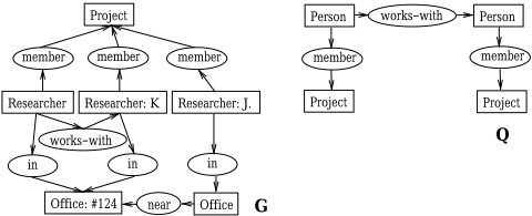
In the drawing of a SG, concept nodes are represented by rectangles and relation nodes by ovals. Generic markers are omitted. And since in our examples we use binary relations only, numbers on edges are replaced by directed edges: a relation node is incident to exactly one incoming and one outgoing edge. Fig. 1 shows two (connected) simple graphs assumed to be defined over the same support.

Simple graphs correspond to the existential conjunctive and positive fragment of FOL (by the semantics ✞ ). Types are mapped to predicates and individual markers to constants. A set of formulas ✞ ✎ ❆ ✢ is assigned to any support ☎ , translating partial orders on types. Given any SG ✮ , a formula ✞ ✎ ✮ ✢ is built as follows. A term is assigned to each concept node: a distinct variable for each generic node, and the constant corresponding to its marker otherwise. An atom ❇ ✎ ❁ ✢ (resp. ❇ ✎ ❁ ❈ ❊ ❊ ❊ ❁ ■ ✢ ) is associated to each concept node (resp. relation node ✺ of arity ❑ ), where ❇ is the type of the node, and ❁ (resp. ❁ ✸ ) is the term assigned to this node (resp. assigned to ✮ ✸ ✎ ✺ ✢ ). Let ◆ ✎ ✮ ✢ be the conjunction of these atoms. ✞ ✎ ✮ ✢ is the existential closure of ◆ ✎ ✮ ✢ . E.g. the formula assigned to the dashed subgraph of ✮ in Fig. 1 is ❖ a80 ❖ ❙ ✎ ❚ ❯ ❲ ❯ ❳ ✺ ❁ ❩ ❯ ✺ ✎ a80 ✢ ❭ ❪ ✺ ❴ ❵ ❯ ❁ ❇ ✎ ❙ ✢ ❭ ❚ ❯ ❲ ❯ ❳ ✺ ❁ ❩ ❯ ✺ ✎ ❛ ✢ ❭ ❅ ❯ ❅ ❝ ❯ ✺ ✎ a80 ✔ ❙ ✢ ❭ ❅ ❯ ❅ ❝ ❯ ✺ ✎ ❛ ✔ ❙ ✢ ❭ works-with ✎ a80 ✔ ❛ ✢ ✢ .

Definition 3 (Projection) Let ✠ and ✮ be two SGs defined on a support ☎ , a projection from ✠ into ✮ is a mapping ✐ from ✰ ✒ ✎ ✠ ✢ to ✰ ✒ ✎ ✮ ✢ and from ✰ ✗ ✎ ✠ ✢ to ✰ ✗ ✎ ✮ ✢ that preserves edges and may decrease node labels:

1. ❧ ❁ ✺ ✧ ✲ ✎ ✠ ✢ ✔ ✐ ✎ ❁ ✢ ✐ ✎ ✺ ✢ ✧ ✲ ✎ ✮ ✢ ; and if ❁ ✍ ✠ ✸ ✎ ✺ ✢ , then ✐ ✎ ❁ ✢ ✍ ✮ ✸ ✎ ✐ ✎ ✺ ✢ ✢ ;
2. ❧ a80 ✧ ✰ ✎ ✠ ✢ ✔ ✵ ✎ ✐ ✎ a80 ✢ ✢ a115 ✵ ✎ a80 ✢ (if a80 is a concept node, a115 is the product of the orders on ✏ ✒ and ✙ ★ ✪ ✤ ✬ , i.e. ❇ ❙ ✇ ❯ ✎ ✐ ✎ a80 ✢ ✢ a115 ❇ ❙ ✇ ❯ ✎ a80 ✢ and ❅ ❳ ✺ ❑ ❯ ✺ ✎ ✐ ✎ a80 ✢ ✢ a115 ❅ ❳ ✺ ❑ ❯ ✺ ✎ a80 ✢ ✢ .

We note ✠ ③ ✮ (✠ subsumes ✮ ) if there exists a projection from ✠ into ✮ . Typically, ✠ represents a query, ✮ a fact, and projections from ✠ to ✮ define answers to ✠ . In Fig. 1, suppose Researcher a115 Person, then there is one projection from ✠ into ✮ . The image of ✠ by this projection is the dashed subgraph of ✮ . Projection is sound and complete w.r.t. the semantics ✞ , up to a normality condition for completeness; the normal formof a SG ✮ is the SGnf ✎ ✮ ✢ obtained by merging concept nodes having the same individual marker. This SG always exists (and is computable in linear time with a naive algorithm). Then: let ✠ and ✮ be two ❆ ✮ s. ✠ ③ nf ✎ ✮ ✢ ⑥ ✞ ✎ ☎ ✢ ✔ ✞ ✎ ✮ ✢ ⑦ ✞ ✎ ✠ ✢ [Chein and Mugnier, 1992], [Gosh andWuwongse, 1995].

For the sake of brevity, we consider in what follows that SGs (and more complex constructs built upon SGs) are given in normal form, and put into normal form if needed after a modification. And, since a SG needs not be a connected graph, we confuse a set of SGs with the SG obtained by performing the disjoint union of its elements. In following definition for instance, the SG ✆ represents a set of SGs.

Definition 4 ( ☎ ✆ Deduction) Let ✆ and ✠ be two SGs. ✠ can be deduced from ✆ if ✠ ③ ✆ .

The ☎ ✆ deduction problem is NP-complete [Chein and Mugnier, 1992]. Note that the subsumption relation induced by projection over SGs is a quasi-order. Two graphs are said to be equivalent if they project to each other. A SG is said to be redundant if it is equivalent to one of its strict subgraphs. Redundancy checking is an NP-complete problem. Each equivalence class admits a unique (up to isomorphism) non redundant graph [Chein and Mugnier, 1992].

3 Overview of the ☛ ☞ Family

From a modeling viewpoint, the simple graphs model has two essential properties. The objects, simple graphs, are easily understandable by an end-user (a knowledge engineer, or even an expert). And reasonings are easily understandable too, for two reasons: projection is a graph matching operation, thus easily interpretable and visualisable; and the same language is used at interface and operational levels. It follows that reasonings can be explained in a natural manner to the user, step by step, and directly on his own modelization (see for instance the knowledge engineering application described in [Bos et al., 1997] or experiments in document retrieval done by [Genest, 2000], where in both cases the representation language is at the expert level). The ☎ ✆ family keeps these essential properties.

Let us now informally present the most general model of the family. Throughout this section, we will use examples inspired from a modelization of a knowledge acquisition case study, called Sysiphus-I: it describes a resource allocation problem, where the aim is to assign offices to persons of a research group while fulfilling constraints [Baget et al., 1999].

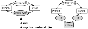
Simple graphs are the basic constructs, upon which more complex constructs, rules and constraints, are defined, and operations are based on projection. A rule expresses a knowledge of form "if ⑨ holds then ⑩ can be added". It is encoded into a simple graph provided with two colors, highlighting the hypothesis and the conclusion of the rule. In drawings, we represent the hypothesis by white nodes, and the conclusion by gray ones. Rules are used in the following way: if the hypothesis of a rule can be projected into a graph, then the rule is applicable to the graph, and its conclusion can be added to the graph according to the projection. The rule of Fig. 2 can be understood as "for all persons a80 and ❙ , if a80 works with ❙ , then ❙ works with a80 ". It can be applied to ✮ of Fig. 1, adding a relation node (work-with) with predecessor [Researcher: K] and successor [Researcher].

A constraint can be a positive constraint or a negative constraint, expressing a knowledge of form "if ⑨ holds, so must ⑩ ", or "if ⑨ holds, ⑩ must not". It is also a bicolored simple graph: the first color defines the condition part, and the second color the mandatory (or forbidden) part. A graph ✮ satisfies a positive constraint ❶ if each projection from the condition part of ❶ into ✮ can be extended as a projection of the whole ❶ . And ✮ satisfies a negative constraint if no projection of ❶ into ✮ can be extended as a projection of the whole ❶ . Fig. 2 represents the negative constraint "two persons working together should not share an office". The graph ✮ of Fig 1 does not satisfy this constraint because "there is a researcher who works with researcher K" (projection of the condition part of ❶ ) "and they share office #124" (extension of the projection to a projection of the whole ❶ ).

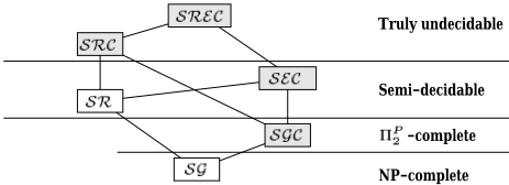
duced from ✟ (we note ✠ ③ ✟ ). If we impose some of the sets ❷ , ❸ or ❹ to be empty, one obtains specific reasoning models. Note that in the absence of constraints (❹ ✍ ➄ ), inference and evolution rules have the same behavior, thus ❷ and ❸ can be confused. The ☎ ✆ family is then composed of the six following models.

• ➆ the ☎ ✆ model for ✟ = ✎ ✆ ✔ ➄ ✔ ➄ ✔ ➄ ✢
• ➆ the ☎ ❷ model for ✟ = ✎ ✆ ✔ ❷ ✔ ❸ ✔ ➄ ✢
• ➆ the ☎ ✆ ❹ model for ✟ = ✎ ✆ ✔ ➄ ✔ ➄ ✔ ❹ ✢
• ➆ the ☎ ❷ ❹ model for ✟ = ✎ ✆ ✔ ❷ ✔ ➄ ✔ ❹ ✢
• ➆ the ☎ ❸ ❹ model for ✟ = ✎ ✆ ✔ ➄ ✔ ❸ ✔ ❹ ✢
• ➆ the ☎ ❷ ❸ ❹ model for ✟ = ✎ ✆ ✔ ❷ ✔ ❸ ✔ ❹ ✢

Since a fact has the same semantics as a rule with an empty hypothesis, the set ✆ is only used inmodels names when both rule sets ❷ and ❸ are empty. The hierarchy of these models is represented in Fig. 3. It highlights the decidability and complexity of the associated deduction problems.

When constraints are involved, we distinguish between two kinds of rules: inference rules of form "if ⑨ then add ⑩ " and evolution rules of form "if ⑨ then add ⑩ , except if it brings inconsistency". Now, a knowledge base contains four sets representing different kinds of knowledge: a set ✆ of simple graphs encoding factual knowledge, a set ❷ of inference rules, a set ❸ of evolution rules and a set ❹ of constraints. PSfrag replacements

Let us outline the deduction problem: the problem takes in input a knowledge base (KB) and a goal expressed as a SG, and asks whether there is a path of consistent worlds evolving from the initial one to a world satisfying the goal. Factual knowledge describes an initial world; inference rules represent implicit knowledge about worlds; evolution rules represent possible transitions from one world to other worlds; constraints define consistency of worlds; a successor of a consistent world is obtained by an evolution rule application; solving the problem consists in finding a path of consistent worlds evolving from the initial one to a world satisfying the goal.

In the particular case of the Sysiphus-I modelization, ✆ and ❷ describe initial information (office locations, persons and group organization), ❹ represents allocation constraints, ❸ consists of one evolution rule: "whenever there are a person and an office, try to assign this office to this person". The goal represents a situation where each person of the group has an office. A solution to the problem is a world obtained from the initial one by a sequence of office assignments, where each person has an office, while satisfying allocation constraints.

Let us now specify definitions and notations concerning the ☎ ✆ family. Rules and constraints are defined as colored SGs.

Definition 5 (colored SGs) A colored simple graph is a pair ❛ ✍ ✎ ✮ ✔ ❺ ✢ where ✮ is a SG and ❺ is a mapping from ✰ ✎ ✮ ✢ into ✪ ❻ ✔ ❼ ✬ . The number associated to a node is called the color of the node. We denote by ❛ ❽ ✸ ❾ the subgraph of ✮ induced by ✽ -colored nodes. The subgraph ❛ ❽ ❿ ❾ must form a SG (i.e. the neighbors of a relation node of the hypothesis must also belong to the hypothesis).

A KB is denoted by ✟ ✍ ✎ ✆ ✔ ❷ ✔ ❸ ✔ ❹ ✢ . Given a KB ✟ and a goal ✠ , the deduction problem asks whether ✠ can be de-

4 SGs and Rules: the ☛ ➒ Model

A simple graph rule (SG rule) embeds knowledge of form "if ⑨ then ⑩ ". The following definition is equivalent to the more traditional one (two SGs related with coreference links) used in [Gosh and Wuwongse, 1995; Salvat, 1998].

Definition 6 (SGRules) A simple graph rule ❚ is a colored SG. ❚ ❽ ❿ ❾ is called its hypothesis, and ❚ ❽ ❈ ❾ its conclusion.

Deduction depends on the notion of a rule application: it is a graph transformation based upon projection.

Definition 7 (Application of a SGRule) Let ✮ be a SG, and ❚ be a SG rule. ❚ is applicable to ✮ if there exists a projection, say ✐ , from ❚ ❽ ❿ ❾ (the hypothesis of ❚ ) into ✮ . In that case, the result of the application of ❚ on ✮ according to ✐ is the graph ✮ ➔ obtained by making the disjoint union of ✮ and of a copy of ❚ ❽ ❈ ❾ (the conclusion of ❚ ), then, for every edge ❁ ✺ , where ❁ ✧ ❚ ❽ ❿ ❾ and ✺ ✧ ❚ ❽ ❈ ❾ , adding an edge with the same number between ✐ ✎ ❁ ✢ and the copy of ✺ . ✮ ➔ is said to be an immediate ❚ -derivation from ✮ .

A derivation is naturally defined as a (possibly empty) sequence of rule applications:

Definition 8 (Derivation) Let ❷ be a set of SG rules, and ✮ be a SG. We call ❷ -derivation from ✮ to a SG ✮ ➔ a sequence of SGs ✮ ✍ ✮ ❿ ✔ ❊ ❊ ❊ ✔ ✮ ■ ✍ ✮ ➔ such that, for ❼ a115 ✽ a115 ❑ , ✮ ✸ is an immediate ❚ -derivation from ✮ ✸ → ❈ , where ❚ ✧ ❷ .

To deduce a SG ✠ , we must be able to derive a SG into which ➣ ✠ can be projected, hence the following definition:

Definition 9 (Deduction in ☎ ❷ ) Let ✟ ✍ ✎ ✆ ✔ ❷ ✢ be a KB and let ✠ be a SG. ✠ can be deduced from ✟ (notation ✠ ③ ✎ ✆ ✔ ❷ ✢ ) if there exists an ❷ -derivation from ✆ to a SG ➙ such that ✠ ③ ➙ .

The semantics ✞ is extended to translate SG rules: let ❚ ❿ and ❚ ❈ be two SGs, s.t. ❚ ❿ ✍ ❚ ❽ ❿ ❾ and ❚ ❈ is the SG obtained from ❚ ❽ ❈ ❾ by adding the neighbors of the relation nodes of ❚ ❽ ❈ ❾ which are concept nodes of ❚ ❽ ❿ ❾ . Then ✞ ✎ ❚ ✢ ✍ ❧ a80 ❈ ❊ ❊ ❊ a80 ➞ ✎ ◆ ✎ ❚ ❿ ✢ ➟ ❖ ❙ ❈ ❊ ❊ ❊ ❙ ➠ ◆ ✎ ❚ ❈ ✢ ) where a80 ✸ are the variables of ◆ ✎ ❚ ❿ ✢ and ❙ ➢ are the variables of ◆ ✎ ❚ ❈ ✢ that do not appear in ◆ ✎ ❚ ❿ ✢ . The following soundness and completeness result is obtained: ✠ ③ ✎ ✆ ✔ ❷ ✢ ⑥ ✞ ✎ ☎ ✢ ✔ ✞ ✎ ✆ ✢ ✔ ✞ ✎ ❷ ✢ ⑦ ✞ ✎ ✠ ✢ [Salvat, 1998]. The ☎ ❷ deduction problem is semi-decidable [Coulondre and Salvat, 1998].

5 SGs and Constraints: the ☛ ☞ ➥ Model

Let us now introduce constraints, which are used to validate knowledge. In presence of constraints, deduction is defined only on a consistent knowledge base.

Definition 10 (Constraints) A positive (resp. negative) constraint ❶ is a colored SG. ❶ ❽ ❿ ❾ is called the trigger of the constraint, ❶ ❽ ❈ ❾ is called its obligation (resp. interdiction). A SG ✮ ✐ -violates a positive (resp. negative) constraint ❶ if ✐ is a projection of the trigger of ❶ into the non redundant form of ✮ (resp. into ✮ ) that cannot be extended (resp. that can be extended) to a projection of ❶ as a whole. ✮ violates ❶ if it ✐ -violates ❶ for some projection ✐ . Otherwise, ✮ satisfies ❶ .

Notice there may be two equivalent SGs, such that one satisfies a positive constraint and the other does not. E.g. given a constraint ❶ , take ✮ satisfying ❶ , and the equivalent (redundant) graph ➙ obtained by making the disjoint union of ✮ and the trigger of ❶ . ➙ violates ❶ . We have thus chosen to define constraint satisfaction w.r.t. the non redundant form of a SG. This problem does not occur with negative constraints.

Two constraints ❶ ❈ and ❶ ➧ are said equivalent if, for every graph ✮ , ✮ violates ❶ ❈ iff ✮ violates ❶ ➧ . Any negative constraint ❶ is equivalent to the negative constraint obtained from ❶ by coloring all its nodes by 1. Furthermore, negative constraints are indeed a particular case of positive ones: consider the positive constraint ❶ ➔ obtained from a negative one ❶ by coloring all nodes of ❶ by 0, then adding a concept node typed NotThere, colored by 1, where NotThere is incomparable with all other types and does not appear anywhere excepted in ❹ . Then a graph ✮ violates ❶ if and only if it violates ❶ ➔ . Positive constraints strictly include negative constraints, in the sense that the associated consistency problems are not in the same complexity class (see theorem 3).

Let us relate our definitions to other definitions of constraints found in the CG literature. The constraints of [Mineau and Missaoui, 1997] correspond to a particular case of our constraints where the trigger and the obligation are not connected. In turn, our constraints are a particular case of the minimal descriptive constraints of [Dibie et al., 1998], where the disjunctive part is restricted to one graph.

Definition 11 (Consistency/Deduction in ☎ ✆ ❹ ) A KB ✟ ✍ ✎ ✆ ✔ ❹ ✢ is consistent if ✆ satisfies all constraints of ❹ . A SG ✠ can be deduced from ✟ if ✟ is consistent and ✠ can be deduced from ✆ .

Note that a ✠ that violates a constraint of ✟ may still be deduced from ✟ . It does not matter since ✠ is a partial representation of knowledge deducible from ✟ . How can we translate the notion of consistency into FOL? For negative constraints, the correspondence is immediate, and relies on projection soundness and completeness.

Theorem 1 A SG ✮ violates a negative constraint ❶ ✍ ✎ ❶ ➔ ✔ ❺ ✢ iff ✞ ✎ ☎ ✢ ✔ ✞ ✎ ✮ ✢ ⑦ ✞ ✎ ❶ ➔ ✢ , where ❶ ➔ is the SG underlying ❶ .

Consistency relative to positive constraints can be explained with FOL, translating "projection" into a notion of logical "substitution" between the formulas associated to graphs (see for instance the S-substitution of [Chein and Mugnier, 1992]). Another bridge can be built using rules. Indeed, a graph ✮ satisfies a positive constraint ❶ if and only if, considering ❶ as a rule, all applications of ❶ on ✮ produce a graph equivalent to ✮ . Or, more specifically:

Property 1 A SG ✮ ✐ -violates a positive constraint ❶ iff, considering ❶ as a rule, the application of ❶ on ✮ according to ✐ produces a graph not equivalent to ✮ .

Using soundness and completeness of the ☎ ❷ deduction, and property 1, one obtains the following relation with FOL:

Theorem 2 A SG ✮ violates a positive constraint ❶ iff there is a SG ✮ ➔ such that ✞ ✎ ☎ ✢ ✔ ✞ ✎ ✮ ✢ ✔ ✞ ✎ ❶ ✢ ⑦ ✞ ✎ ✮ ➔ ✢ and not ✞ ✎ ☎ ✢ ✔ ✞ ✎ ✮ ✢ ⑦ ✞ ✎ ✮ ➔ ✢ , where ✞ ✎ ❶ ✢ is the translation of ❶ considered as a rule.

The problem "does a given graph satisfy a given constraint?" is co-NP-complete if this constraint is a negative constraint (we must check the absence of projection), but becomes ➭ ➯ ➧ -complete for a positive one (➭ ➯ ➧ is co-NP NP ).

Theorem 3 (Complexity in ☎ ✆ ❹ ) Consistency in ☎ ✆ ❹ is ➭ ➯ ➧ -complete (but is co-NP-complete if all constraints are negative).

Sketch of proof: ☎ ✆ ❹ -Consistency belongs to ➭ ➯ ➧ since it corresponds to the language ➲ ✍ ✪ a80 ➳ ❧ ❙ ❈ ❖ ❙ ➧ ❚ ✎ a80 ✔ ❙ ❈ ✔ ❙ ➧ ✢ ✬ , where a80 encodes an instance ✮ ➵ ❶ and ✎ a80 ✔ ❙ ❈ ✔ ❙ ➧ ✢ ✧ ❚ iff ❙ ❈ is a projection ➭ ❿ from ❶ ❽ ❿ ❾ into ✮ , ❙ ➧ is a projection ➭ from ❶ into ✮ s.t. ➭ ➸ ❶ ❽ ❿ ❾ ➺ ✍ ➭ ❿ . Now, let us consider the ➭ ➯ ➧ -complete problem ⑩ ➻ ➧ : given a boolean formula ✲ , and a partition ✪ ➼ ❈ ✔ ➼ ➧ ✬ of its variables, is it true that for any truth assignment for the variables in ➼ ❈ there exists a truth assignment for the variables in ➼ ➧ s.t. ✲ is true? We first show that the special case where ✲ is an instance of 3-SAT remains ➭ ➯ ➧ -complete (let us call this problem 3-SAT➻ ➧ ). For that we use the polynomial transformation from any boolean formula to a set of clauses described in ([Papadimitriou, 1994], example 8.3), followed by a polynomial transformation from a clause to clauses with 3 literals. The "new" variables are put in the set ➼ ➧ . We then reduce 3-SAT ➻ ➧ to ☎ ✆ ❹ -Consistency. ✲ is mapped to a constraint ❶ : briefly said, there is one concept node [t:*] for each variable and one ternary relation node with type ✺ ✸ for each clause ❁ ✸ . ❶ ❽ ❿ ❾ is composed of all concept nodes coming from variables in ➼ ❈ . ✮ is composed of two individual concept nodes [t:0] and [t:1] corresponding to the truth values and, for each clause ❁ ✸ there is one relation node of type ✺ ✸ for each triple of truth values giving the value true to ❁ ✸ . Note that, since ❶ ❽ ❿ ❾ does not contain any relation node, any truth assignment for the variables of ➼ ❈ is a projection from ❶ ❽ ❿ ❾ to ✮ , and reciprocally. ➽

Corollary 1 Deduction in ☎ ✆ ❹ is ➭ ➯ ➧ -complete.

Note that the theorem 3 can be used to show that consistency of minimal descriptive constraints in [Dibie et al., 1998] is also ➭ ➯ ➧ -complete.

6 Rules and Constraints: ☛ ➾ ➥ ➚ ☛ ➒ ➥

The two kinds of rules, inference rules ❷ and evolution rules ❸ , define two alternativemodels. In ☎ ❸ ❹ , ✆ is seen as the initial world, root of a potentially infinite tree of possible worlds, and ❸ describes the possible evolutions from one world to others. The deduction problem asks whether there is a path of consistent worlds from ✆ to a world satisfying ✠ .

Definition 12 (Deduction in ☎ ❸ ❹ ) Let ✟ ✍ ✎ ✆ ✔ ❸ ✔ ❹ ✢ be a KB, and let ✠ be a SG. ✠ can be deduced from ✟ if there is an ❸ -derivation ✆ ✍ ✮ ❿ ✔ ❊ ❊ ❊ ✔ ✮ ■ such that, for ❻ a115 ✽ a115 ❑ , ✎ ✮ ✸ ✔ ❹ ✢ is consistent and ✠ can be deduced from ✮ ■ .

In ☎ ❷ ❹ , ✆ provided with ❷ is a finite description of a potentially infinite world, that has to be consistent. Applying a rule to ✆ can create inconsistency, but a further application of a rule may restore consistency. Let us formalize this notion of consistency restoration. Suppose there is a ✐ -violation of a positive constraint ❶ in ✆ ; this violation ✎ ❶ ✔ ✐ ✢ is said to be ❷ -restorable if there exists an ❷ -derivation from ✆ into ✮ ➔ such that the projection ✐ of the trigger of ❶ into ✮ ➔ can be extended to a projection of ❶ as a whole. The violation of a negative constraint can never be restored. Note that the ❷ -restoration can create newviolations, that must themselves be proven ❷ -restorable.

Definition 13 (Consistency/Deduction in ☎ ❷ ❹ ) A KB ✟ ✍ ✎ ✆ ✔ ❷ ✔ ❹ ✢ is consistent if, for any SG ✮ ➔ that can be ❷ -derived from ✆ , for every constraint ❶ ✧ ❹ , for every ✐ -violation of ❶ in ✮ ➔ , ✎ ❶ ✔ ✐ ✢ is ❷ -restorable. A SG ✠ can be deduced from ✟ if ✟ is consistent and ✠ can be deduced from ✎ ✆ ✔ ❷ ✢ .

Consider for instance a KB containing the SG ✮ in Fig. 4, expressing the existence of the number 0, a constraint and a rule, both represented by the colored SG ❛ . The constraint asserts that for every integer ➶ , there must be an integer ➶ ➔ , successor of ➶ . If the rule is an evolution rule, ✮ is seen as an inconsistent initial world (there is no successor of 0 in ✮ ) and nothing will be deduced from this KB. If the rule is an inference rule, its application immediately repairs the constraint violation, while creating a new integer, that has no successor, thus a new violation. Finally, every constraint violation could eventually be repaired by a rule application, and the KB should be proven consistent.

Let us point out that the ☎ ❷ model is obtained from ☎ ❷ ❹ or ☎ ❸ ❹ when ❹ is empty, and ☎ ✆ ❹ is obtained from ☎ ❷ ❹ (resp. ☎ ❸ ❹ ) when ❷ (resp. ❸ ) is empty.

Theorem 4 (Complexity in ☎ ❸ ❹ ✥ ☎ ❷ ❹ ) Deduction in ☎ ❸ ❹ is semi-decidable. Consistency and deduction in ☎ ❷ ❹ are truly undecidable.

Proof: ☎ ❸ ❹ includes ☎ ❷ thus ☎ ❸ ❹ -deduction is not decidable. When ✠ is deducible from ✟ , a breadth-first search of the tree of all derivations from ✟ , each graph being checked for consistency, ensures that ✮ ■ is found in finite time. For ☎ ❷ ❹ , we show that checking consistency is truly undecidable. Let ✟ be a KB where ❹ contains a positive constraint ❶ ➹ and a negative constraint ❶ → , both with an empty trigger. For proving consistency, one has to prove that ❶ → ➘ ③ ✎ ✆ ✔ ❷ ✢ , and the algorithm does not stop in this case (from semidecidability of deduction in ☎ ❷ ). The same holds for the complementary problem (proving inconsistency) taking ❶ ➹ instead of ❶ → , hence the undecidability. ➽

7 Combining Inference and Evolution

The ☎ ❷ ❸ ❹ model combines both derivation schemes of the ☎ ❷ ❹ and ☎ ❸ ❹ models. Now, ✆ describes an initial world, inference rules of ❷ complete the description of any world, constraints of ❹ evaluate the consistency of a world, evolution rules of ❸ try to make evolve a consistent world into a new, consistent one. The deduction problem is: can ✆ evolve into a consistent world satisfying the goal?

Definition 14 (Deduction in ☎ ❷ ❸ ❹ ) A SG ✮ ➔ is an immediate ❷ ❸ -evolution from a SG ✮ if there exists an ❷ -derivation from ✮ into ✮ ➔ ➔ and an immediate ❸ -derivation from ✮ ➔ ➔ into ✮ ➔ . An ❷ ❸ -evolution from a SG ✮ to a SG ✮ ➔ is a sequence of SGs ✮ ✍ ✮ ❿ ✔ ❊ ❊ ❊ ✔ ✮ ■ ✍ ✮ ➔ such that, for ❼ a115 ✽ a115 ❑ , ✮ ✸ is an immediate ❷ ❸ -evolution from ✮ ✸ → ❈ . Given a KB ✟ ✍ ✎ ✆ ✔ ❷ ✔ ❸ ✔ ❹ ✢ , a SG ✠ can be deduced from ✟ if there is an ❷ ❸ -evolution ✆ ✍ ✮ ❿ ✔ ❊ ❊ ❊ ✔ ✮ ■ where, for ❻ a115 ✽ a115 ❑ , ✎ ✮ ✸ ✔ ❷ ✔ ❹ ✢ is consistent, and ✠ can be deduced from ✎ ✮ ■ ✔ ❷ ✢ .

When ❸ ✍ ➄ , one obtains the ☎ ❷ ❹ model (there is only one world). When ❷ ✍ ➄ , one obtains ☎ ❸ ❹ (information contained in a world is complete). As a generalization of ☎ ❷ ❹ , deduction in ☎ ❷ ❸ ❹ is truly undecidable. Let us now consider a decidable fragment of ☎ ❷ ❸ ❹ (which in particular was sufficient for the Sysiphus-I modelization). First note a rule has only to be applied once according to a given projection: further applications with this projection obviously produce redundant information. Such applications are said to be useless. A SG ✮ is said to be closed w.r.t. a rule ❚ if all applications of ❚ on ✮ are useless. Given a set of rules ❷ , we note, when it exists, ✮ ❒ ➉ (the closure of ✮ w.r.t. ❷ ) the smallest graph derived from ✮ that is closed w.r.t. every rule in ❷ . When it exists ✮ ❒ ➉ is unique. ❷ is called a finite expansion set (f.e.s.) if, for every SG ✮ , its closure ✮ ❒ ➉ exists (and thus can be computed in finite time). If ❷ is a finite expansion set, the deduction problem in the ☎ ❷ model becomes decidable (but it is not a necessary condition for decidability).

Property 2 (Finite expansion sets) Let ✟ ✍ ✎ ✆ ✔ ❷ ✔ ❹ ✢ be a KB wher ❰ e ❷ is a finite expansion set. Then ✟ is consistent iff ✎ ✪ ✆ ❒ ➉ ✬ ✔ ❹ ✢ is consistent, and a SG ✠ can be deduced from ✎ ✆ ✔ ❷ ✢ iff ✠ can be deduced from ✎ ✪ ✆ ❒ ➉ ✬ ✢ .

The following decidable case is based on property 2.

Property 3 (Decidable case) Deduction in ☎ ❷ ❸ ❹ is semidecidable if ❷ is a f.e.s. and is decidable if ❷ ★ ❸ is a f.e.s.

Proof: Suppose ❷ is a f.e.s. When ✠ can be deduced, one obtains an answer in finite time; we proceed as for ☎ ❸ ❹ (see proof of theorem 4) but consistency checks are done on the graph closure instead of the graph itself. Now, if ❷ ★ ❸ is a f.e.s., ✆ ❒ ➉ a209 ➊ exists, thus the derivation tree is finite, and consistency checks may only cut some parts of this tree. ➽

A rule is said to be range restricted (by analogy with the so-called rules in Datalog, where all variables of the head must appear in the conclusion) if no generic concept node belongs to its conclusion. Then:

Property 4 A set of range restricted rules is a f.e.s.

Proof: Since all graphs are put into normal form, an individual marker appears at most once in a graph. Then the closure of a SG ✮ can be obtained with a derivation of length a210 ✎ ➶ ■ ✢ , where ➶ is the size of ✎ ✮ ✔ ❷ ✢ and ❑ is the greatest arity of a relation type appearing in a rule conclusion. ➽

8 Conclusion

We propose a family of models that can be seen as the basis of a generic modeling framework. Main features of this framework are the following: a clear distinction between different kinds of knowledge, that fit well with intuitive categories, a uniform graph-based language that keeps essential properties of the SG model, namely readability of objects as well as reasonings. We guess this later point is particularly important for the usability of any knowledge based system. In our framework, all kinds of knowledge are graphs easily interpreted, and reasonings can be graphically represented in a natural manner using the graphs themselves, thus explained to the user on its own modelization.

Technical contributions, w.r.t. previous works on conceptual graphs, can be summarized as follows:

• ➆ the representation of different kinds of knowledge as colored SGs: facts, inference rules, evolution rules and constraints.
• ➆ the integration of constraints into a reasoning model; more or less similar notions of a constraint had already been introduced in [Dibie et al., 1998; Mineau and Missaoui, 1997] but were only used to check consistency of a simple graph (as in the ☎ ✆ ❹ model). The complexity of consistency checking was not known.
• ➆ a systematic study of the obtained family of models with a complexity classification of associated consistency/deduction problems.

We established links between consistency checking and FOL deduction. The operational semantics of models including constraints, namely ☎ ❷ ❸ ❹ , ☎ ❷ ❹ and ☎ ❸ ❹ , is easy to understand but there is an underlying non monotonic mechanism whose logical interpretation should require non standard logics. The definition of a logical semantics for these models is an open problem.

Acknowledgments

We are indebted to Genevi`eve Simonet for her careful reading and some error corrections on an earlier version of this paper, and to Michel Chein, as well as the anonymous reviewers, for their helpful comments.