Leveraging Data About Users in General in the Learning of Individual User Models

1 Introduction

Machine learning techniques are being used increasingly in the development of interactive systems that adapt to individual users. Two contrasting approaches can be distinguished:

• Learning general user models: A system processes observations acquired from a sample of users so as to learn a model that applies to users in general (see, e.g., [Walker et al., 2000]).
• Learning individual user models: While a user ✁ is operating a system ✂ , ✂ processes observations about ✁ so as to learn a model of this particular ✁ (see, e.g., [Segal and Kephart, 1999]).

Each of these types of learning has its own typical benefits, which will be discussed later in this paper. A natural strategy is to combine the advantages of general and individual models: Learn a general user model which can be applied to a new user; adapt the model to each user during the interaction.

✄ This research was supported by the German Science Foundation (DFG) in its Collaborative Research Center on Resource-Adaptive Cognitive Processes, SFB 378, Project B2 (READY). The experiment described in Section 2 was conducted in collaboration with Barbara Großmann-Hutter, Christian M¨uller, and Ralf Rummer. The suggestions of the three anonymous reviewers led to significant improvements. The first author is currently at DFKI, Saarbr¨ucken.

One broad approach that applies this strategy is collaborative filtering, which has been applied widely in systems that recommend products (such as CDs) to users (see, e.g., [Herlocker et al., 1999]). Here, the "general model" is essentially just the database of ratings (or other actions) that have been contributed by users so far. A system could predict how a given user ✁ will rate a given object simply on the basis of this general model, by computing the average of all ratings given for that object. Instead, of course, collaborative filtering systems usually make individualized predictions that are based on the ratings of a subset of users who are especially similar to ✁ .

Although collaborative filtering systems have been highly successful, there are some application scenarios in which it is desirable to learn a more interpretable type of user model, in which causal relationships among variables are represented explicitly. For example, a system ✂ may need to predict how the behavior of the user ✁ will be influenced by particular contextual factors; or it may need to make uncertain inferences about unobserved contextual factors on the basis of ✁ 's behavior. Collaborative filtering is less straightforwardly applicable to this type of problem than another popular type of model: Bayesian networks (BNs). 1

The main issue addressed in the present paper is: How can systems that employ Bayesian networks to model users most effectively exploit data about users in general and data about the current individual user?

Our investigation makes use of data from a controlled experiment.

2 Brief Description of Experiment

We begin by briefly summarizing the methods and results of the experiment (see [M¨uller et al., 2001] for a more complete account). The experimental environment simulated on a computer workstation a situation in which a user is navigating through a crowded airport terminal while asking questions to a mobile assistance system via speech. In each trial, a picture appeared in a corner of the computer screen, and the subject was to introduce and ask a question related to the picture (e.g.,

1 Explanations of Bayesian networks can be found in many sources, including the classic book by Pearl [1988]. An early survey of their application to user modeling was given by Jameson [1996].

"I'm getting thirsty. Will it be possible to get a beer on the plane?").

Two independent variables were manipulated orthogonally:

• TIME PRESSURE?: Whether the subject was instructed (a) to finish each utterance as quickly as possible or (b) to create an especially clear and comprehensible utterance, without regard to time.
• SECONDARY TASK?: Whether or not the subject was required to "navigate" through the terminal depicted on the screen by pressing arrow keys in order to move the cursor on the screen, avoiding obstacles in the process.

In each of the 4 (☎ ✆ ☎ ) conditions, each of the 32 subjects produced 20 utterances. There are therefore 80 "observations" of each subject.

The subjects' speech input was later coded semiautomatically with respect to a wide range of features, including pauses, length, quality of content, and various types of disfluency. For the present study of learning methods, we selected a representative subset of four speech-related variables:

• ARTICULATION RATE: The number of syllables articulated per second of speaking time, not including silent pauses.
• NUMBER OF SYLLABLES: The number of syllables in the utterance.
• DISFLUENCIES: A binary variable that takes the value "True" when any one of four types of disfluency (e.g., starting a sentence but failing to complete it) is present in the utterance.
• SILENT PAUSES: The total duration of the silent pauses in the utterance, relative to the length of the utterance in words.

The practical relevance of this experiment lies mainly in the prospect that a mobile assistance system could interpret the features of a user's speech to make inferences about ✁ 's current psychological state ([M¨uller et al., 2001]). In addition, there are situations in which it can be useful for ✂ to be able to predict particular features of ✁ 's speech in a given situation-for example, so as to determine whether to request input via speech or via another modality.

3 Method andModel Types

The basic BN structure used for the models developed for the experiment is shown in the top two rows of Figure 1. We wish to simulate a situation in which a system ✂ is interactingwith a user ✁ in this experimental situation and obtaining successive observations about ✁ . We will introduce four types of model, each of which will be tested according to the same procedure, which is shown in Table 1.

The characteristics of the four model types are summarized in Table 2; some further comments follow:

The general model is learned from the experimental data via the usual maximum-likelihood method for learning fully observable Bayesian networks (see, e.g., [Buntine, 1996]): The estimate of each (conditional) probability is computed simply in terms of the (relative) frequencies in the data. During the application to an individual user, the model is not adapted further: Essentially, a fresh copy of the model is used

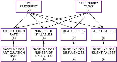
(The four variables in the bottom row are included only in the parametrized model. The number in parentheses for each variable is the number of states of that variable.)

for the prediction of each observation.

The parametrized model is initially learned in the same way as the general model, except that the four parameter variables shown in the bottom row of Figure 1 are included. Each of these variables represents the mean value of the corresponding variable above it for the user in question.

The adaptive model makes use of the AHUGIN ("adaptive HUGIN") method that was introduced by Olesen et al. [1992]. In contrast to the parametrizedmodel, there is no explicit representation of the dimensions along which users may differ. Instead, the probabilities in the conditional probability tables (CPTs) of the BN are adapted whenever a new observation is processed. In this way, a great variety of individual differences can be adapted to, without any need for the designer of the BN to anticipate the nature of these differences. One question that arises in the application of the AHUGIN method concerns the speed with which the CPTs should adapt to the individual user. One simple approach, which is frequently used in other contexts, is to specify for the entire BN a single parameter, called the equivalent sample size (ESS); the ESS essentially represents the extent of the system's reliance on the initial general model, relative to the new data that will be obtained for each user. As we will see below, it is in general not obvious a priori what the most appropriate ESS for a given BN is. Moreover, the optimal value of the ESS can be quite different for different parts of the BN; in the context of our experiment, we may need a different ESS for each combination of a speech variable (e.g., NUMBER OF SYLLABLES) and an experimental condition. One original contribution of this paper is a principled method of estimating the optimal ESSs on the basis of the data collected with previous users. Application of this method yields a BN in which the various parts of the variables' CPTs adapt at different rates to each new user; hence the name differential adaptation. This method is described in detail in the Appendix.

The purely individual model is simply learned entirely on the basis of data from the current subject. So that some sort of inference can be performed right from the start, each CPT is initialized with uniform distributions. But as soon as the first observation for a given configuration of the values of the parent variables TIME PRESSURE? and SECONDARY TASK? has been

Initial model

• A BN defined in the way specified for type T (see Table 2) on the basis of the data from the other subjects in the experiment

Preparation of the test data

1. Determine a single random ordering of the 80 experimental stimuli, to be employed for all users
2. For each individual user U, select the 80 observations for U according to this ordering

Testing the model for a single user U with respect to a variable V

For each observation O in the set of observations for U,

1. Derive a belief about O:
2. Instantiate all variables for O other than V
3. Evaluate the BN to arrive at a belief regarding V
4. Determine the quadratic loss of the derived belief with respect to the actual value of V
5. Learn from the observation:
6. Use the values of all of the variables for the observation O to adapt the model, in the way specified for this type of model (see Table 2)

Presentation of results

• In each curve in a graph, the quadratic loss for each observation is aggregated over all subjects in the experiment
• Moreover, each value plotted is the mean quadratic loss for a block of 8 observations

Otherwise, sharp random fluctuations from one observation to the next would make it difficult to recognize general trends visually

Table 1. Procedure for evaluating the learning (if any) and performance of a model of type T.

Learning From Previous Users Adaptation During Use by the

Current User

General Model

Learned on the basis of all observations of other subjects in the experiment, with no variables for individual parameters No adaptation during use

Parametrized Model

Learned on the basis of all observations of other subjects, with variables for individual parameters The BN is built up as a dynamic BN, a new time slice being created for each observation; parameter nodes are updated as static nodes

Adaptive Model

Individual models are learned for the other subjects as with the purely general model; on the basis of these models, an initial model for U is created that includes an equivalent sample size (ESS) for each configuration of values of parent variables in each conditional probability table (CPT)

After each observation, the CPT entries for the instantiated configurations of values of parent variables are updated according to the AHUGIN algorithm, using the ESS computed for that configuration

Individual model

No prior learning: In the initial model for U, for each parent configuration in each CPT the probabilities are uniformly distributed and a minimal ESS of .0001 is specified Adaptation is done as for the adaptive model, but the same minimal ESS is used for all parent configurations

Table 2. Overview of the four model types compared.

obtained, the initial model has essentially no further impact on the corresponding part of the CPT in question.

4 Results

We will now look at the results for these four models for each of the variables in the experiment. We first consider the four dependent variables in the second row of Figure 1, which need to be predicted by the model. Then we turn to the two independent variables in the top row. The derivation of a belief about one of these variables is essentially a classification task for the system: On the basis of an observation, the system attempts to assign ✁ to a given experimental condition.

4.1 Predicting a VariableWith Simple Individual Differences

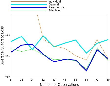
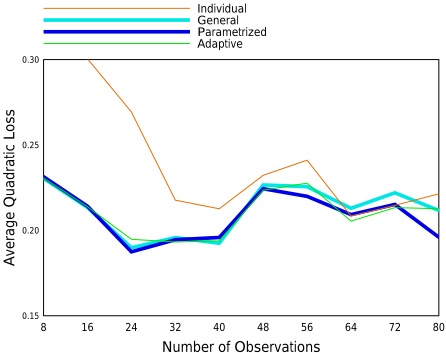
The results for the general model for the variable ARTICULATION RATE are shown by the solid thick curve in Figure 2. First, note that the only reason why this curve is not a straight horizontal line is that there is considerable randomfluctuation in the quadratic loss variable; so there is no point in trying to interpret the individual zig-zags in the curves for the general model.

It is meaningful, on the other hand, to compare the overall performance of the general model with that of the parametrized and the adaptive models. As with all other comparisons that follow, we will use simple sign tests that take into account only the last 24 observations (3 blocks in the figures). 2 Each of these models performs consistently better than the general model during the last 24 observations ( ✟ ✠ ☛ ✌ ✍ ). This fact is understandable given that stable individual differences in articulation rate are known to exist. For this variable, the parametrized and the adaptive models perform very similarly.

2 A test like this reflects how likely it is that a difference between the two curves in question would be found if we made the same comparison again, under the same circumstances and with the same subjects. It does not warrant a generalization to other subjects, tasks, models, etc.

The curve for the individual model shows a pattern that we will see to be typical: At first, the predictions are very inaccurate, as would be expected given that they are initially based on an arbitrary set of probabilities. But after about 30 observations the individual model does as well as the general model; and during the last 24 observations it is somewhat better (✟ ✠ ☛ ✌ ✒ ).

4.2 Predicting a VariableWithMore Complex Individual Differences

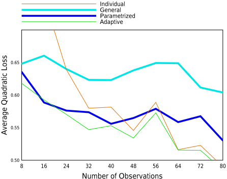
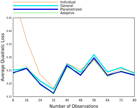
It is likewise generally known that people differ in their verbosity: the amount that they say in any given situation. Figure 3 shows the results for the variable NUMBER OF SYLLABLES. The individual differences are apparently even more important than for ARTICULATION RATE: The individual model catches up with the general model in the third block, and by the last three blocks it is tied for first place.

Moreover, the adaptive model significantly outperforms the parametrizedmodel ( ✟ ✠ ☛ ✌ ☎ for the last 24 observations). Figure 4 helps to explain this advantage by displaying the accuracy levels for each of the four experimental conditions (without showing the time course of learning). The figure shows that the superior performance of the adaptive model occurs in just one of the four experimental conditions: Q✖ , in which subjects were instructed to produce high-quality utterances without having to navigate. Some subjects responded to this condition by creating elaborate, lengthy formulations, while others simply aimed to increase the clarity of an utterance of normal length. It is understandable that these individual differences should be hard to predict in terms of a single dimension of "verbosity", which is what the parametrized model has to use. The ability of the adaptive and individual models to learn ✁ 's behavior in each individual condition proves to be an advantage here. Note also that the ESS employed for the condition Q✖ is lower than that for the other conditions. In effect, the system has noticed that people re- T/Q:

-/+:

Time Pressure / Quality Emphasis

Without / With Navigation

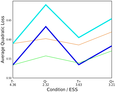
spond very differently to this condition with respect to this variable and that it should therefore base its model largely on what it observes in the individual ✁ 's behavior.

4.3 Predicting Low-Frequency Behaviors

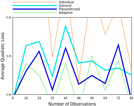
The variable DISFLUENCIES (Figure 5) is an example of a variable for which there is little to be gained through adaptation to the individual user. On the average, only about 1 utterance in 8 contains one or more of the disfluencies in question. Consequently, it is inherently difficult for a system, given a limited number of observations, to acquire a model of a user's tendency to produce disfluencies which is better than the general model-even though stable differences among users might be found, given enough data. This fact is shown by the strong similarity of all four curves during the last few blocks of observations.

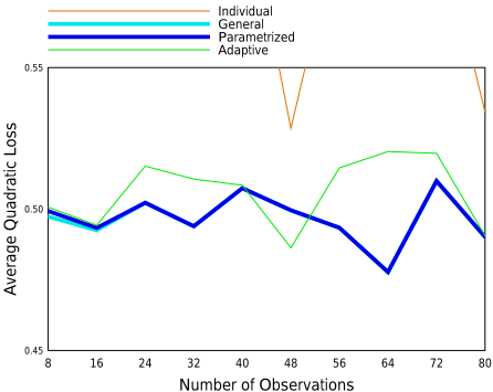
Measurable SILENT PAUSES (Figure 6) within an utterance are also rather infrequent events, occurring only about once in every 5 utterances overall. Still, the parametrized model does manage to outperformthe general model here (✟ ✗ ☛ ✌ ☎ ).

4.4 Inferring the Experimental Condition

Figure 7 shows the results for a classification task: Instead of predicting a particular aspect of ✁ 's behavior, ✂ has to infer whether ✁ was working under time pressure or with an emphasis on quality, given the features of one of ✁ 's utterances and knowledge of the value of the other independent variable (SECONDARY TASK?).

The pattern of relative accuracy shown in the figure is somewhat inconsistent with the pattern shown in the previous figures:

• The individual model never catches up with the other models in terms of accuracy, whereas it had done so for each of the prediction tasks.
• The parametrized and adaptive models do not show a very clear advantage over the general model (✟ ✗ ☛ ✌ ✒ and ✟ ✗ ☛ ✍ ✤ , respectively)-although one might have expected such an advantage, given that these models performed clearly better in the prediction of two of the four speech variables (ARTICULATION RATE and NUMBER OF SYLLABLES).

For classification with regard to SECONDARY TASK? (Figure 8), there are no reliable differences at all except that the individual model is much worse than the others throughout. This particular classification task-determining on the basis of a single utterance whether the subject is navigating or not-is very difficult, with performance being at best marginally above the chance level (which corresponds to a quadratic loss of 0.5).

These results remind us of the general point, argued by previous authors, that there is not necessarily one best model for a given set of data. For example, Friedman et al. [1997] discuss the reasons why a BN that is optimal with respect to some general accuracy criterion may perform suboptimally on classification tasks; and they propose methods for optimizing the classification accuracy of a learned BN. Greiner et al. [1997] have argued more generally that learning should take into account the specific queries that a BN is intended to answer.

5 Discussion

5.1 Overall Comparison of Model Types

Table 3 summarizes the points that have been made in the preceding sections about (a) the theoretical strengths and weaknesses of the four model types, (b) the empirical results for them that were obtained in our experiment, and (c) practical considerations that may be equally important for the choice of a type of model.

The empirical results do not appear to depend on specific properties of this one experiment: When we performed the corresponding analyses for a quite different experiment (described in [Jameson et al., 2001]), a very similar pattern emerged: In particular, for each of the categories of variables discussed in the subsections of the previous section, there was at least one variable in the other experiment that fell into that category and yielded similar results with regard to the performance of the four model types.

Regarding the empirical results: Although the parametrized and adaptive models perform best overall, the general and individual models each show competitive performance

Empirical Results

• Individual differences are never taken into account
• Knowledge about the nature of individual differences can be represented explicitly
• Many parameters may be required if individual differences are complex
• Specific parts of the model are adapted at different rates in a principled manner
• Permits smooth transition from a general model to an individual model
• The number of degrees of freedom for the learning may be unnecessarily high, relative to the paramaterized model, so that learning is unnecessarily slow
• Since no use is made of prior knowledge or data, inference is likely to be very inaccurate during the initial phase of use
• There is no bias against entirely unexpected patterns of behavior

General Model

• Out-performed in the long run by the parametrized and adaptive models, except where individual differences are small or very hard to learn; and sometimes by the individual model

Parametrized Model

• Generally better than the general and individual models and competitive with the adaptive model
• Somewhat poorer than the adaptive or even the individual model when individual differences are complex
• Generally good performance, especially on prediction tasks with complex individual differences

Adaptive Model

Individual model

• Very poor performance during some initial phase of use
• The phase of poor performance is especially long for classification tasks
• Good ultimate prediction performance
• where behavior is highly idiosyncratic
• Ample prior data required
• No overhead for run-time adaptation
• Ample prior data required
• Dynamic Bayesian networks can raise complexity problems
• Parameters can be shared with other user models
• Ample prior data required
• No prior explicit knowledge about individual differences required
• The adaptation mechanism must be invoked repeatedly during system use
• No prior knowledge or data required
• The adaptation mechanism must be invoked repeatedly during system use

Table 3. Overview of the strengths and limitations of the four model types.

under certain conditions. Consequently, one of these models may be turn out to be the most suitable one when these conditions are met and the practical considerations favor the model in question.

The use of Table 3 to select a model type for a given application scenario is made more difficult by the fact that some of the conditions mentioned (e.g. "individual differences are complex") refer to properties of the data that may or may not be known a priori. It may therefore be necessary to test two or more types of model empirically on data from the domain in question before arriving at a decision. Even in these cases, Table 3 should be helpful in that it calls attention to the key considerations and the most promising model types.

5.2 Novel Aspects of the Differential Adaptation Method

The most salient features of the method of differential adaptation are the following:

1. It leverages data about previous users not only to learn an initial general user model but also to learn how fast the various aspects of this model should adapt to each new individual user.
2. It does so without requiring the explicit representation of dimensions along which individual users may differ, as is the case with parametrized models.

As another example of a scenario in which this method might be useful, consider the system Syskill & Webert ([Pazzani and Billsus, 1997]), which predicts whether a given web page will be interesting to the current user. In the main version of the system, the user model consists essentially of a set of probabilities for each word ✦ in a set of relevant words: ✟ ✧ W is present ✩ page is interesting✪ and ✟ ✧ W is present ✩ page is uninteresting ✪ . Pazzani and Billsus note that it can take inconveniently long for the system to learn the necessary probabilities solely on the basis of ✁ 's page ratings, and they propose solutions to this problem. In accordance with the basic idea of differential adaptation, this problem could be dealt with as follows: For each word ✦ , the system would derive a prior expectation (more precisely, a beta distribution), for ✟ ✧ W is present ✩ page is interesting ✪ on the basis of the data of other users, through the procedure described in the Appendix, along with a corresponding expectation for ✟ ✧ W is present ✩ page is uninteresting✪ ; and these expectations would be used and updated as in the tests described above. This method might be especially useful in the case of words that (a) occur infrequently but (b) exhibit similar probabilities for most users.

6 Summary of Contributions

As the learning of user models for adaptive systems becomes more widespread, increasing attention will be devoted to the

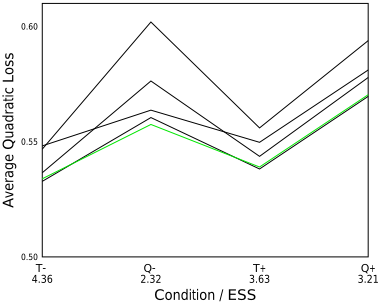
(The solid line shows the results for the adaptive model which were shown in Figure 4; The dashed lines show the results for models using fixed ESSs of 1, 5, 10, and 20, respectively, with the length of the dashes reflecting the ESSs.)

goal of making optimal use of the available data. Focusing on models that take the form of Bayesian networks, this paper has (a) systematically compared, with regard to several criteria, four representative ways of exploiting data about users in general and/or individual users; and (b) introduced a variant of the AHUGIN adaptation method called differential adaptation, which represents a principled way of determining the speed with which the various aspects of a general model should be adapted to an individual user.

A Appendix: The Differential Adaptation Method

As was noted in Section 3, the simplest type of adaptive model that can be realized with AHUGIN is one in which a single equivalent sample size (ESS) is specified for an entire BN. Figure 9 illustrates the limitations of this method: The solid line, which is repeated from Figure 4, shows the predictive accuracy of the adaptive model that used the method of differential adaptation; recall that this model computed and used the four ESSs shown under the x-axis, one for each experimental condition for the variable NUMBER OF SYLLABLES. Each of the dashed lines shows the results for a model that used a constant ESS of 1, 5, 10, or 20, respectively. The results for the ESSs of 1, 10, and 20 are noticeably worse than those for the ESS of 5 and for differential adaptation; that is, the choice of an ESS really does make a difference. The fact that the accuracy for the ESS of 5 is only slightly worse than that for differential adaptation is not surprising, given that the ESSs computed by differential adaptation are fairly close to 5. The main contribution of the differential adaptation method here is to compute the right general level of the ESSs automatically, avoiding the need for trial and error on the part of the designer of the BN. Differential adaptation also gains a bit of additional accuracy by computing a different ESS for each experimental condition, in particular choosing a lower value for the condition "Q-", in which individual differences are especially large (cf. 4.2).

Similarly, for each of the other variables examined in this experiment and the experiment mentioned in 5.1, differential adaptation consistently performed at least as well as the best fixed-ESS model, deriving ESSs ranging from 12.9 to essentially 0. The differences from the fixed-ESS models were in most cases smaller than those shown in Figure 9. Still, since differential adaptation is computationally quite straightforward (see below), there appears to be no reason not to use it whenever it is applicable.

The rest of this Appendix explains in more detail the differential adaptation method and the relevant aspects of the AHUGIN adaptation facility. 3

Suppose that a variable ✬ has ✭ possible states. To simplify notation, all mathematical expressions that follow refer to one particular configuration ✮ of states of the parent variables of ✬ . For this configuration, there are ✭ probabilities ✟ ✯ in the conditional probability table (CPT) for ✬ . In addition to storing these ✭ probabilities, AHUGIN maintains for each ✮ a Dirichlet distribution (see, e.g., [Heckerman, 1995, Section 2]; [Olesen et al., 1992]) that represents the system's current expectation concerning the true vector of probabilities of which ✟ ✯ are simply the current estimates. The parameters of each such Dirichlet distribution are as follows:

• a vector of ✭ means ✲ ✯ ;
• an equivalent sample size (ESS, denoted in the formulas as ✳ ).

The means ✲ ✯ are numerically identical to the ✭ CPT entries ✟ ✯ , but it will be helpful to denote them with ✲ ✯ when we are viewing them as parameters of the Dirichlet distribution.

Whenever a new observation is obtained in which the configuration ✮ of states of ✬ 's parents is realized, ✳ is incremented by 1 and the ✲ ✯ are updated according to the usual method for Dirichlet distributions.

In the context of learning user models, the AHUGIN algorithm gives us the opportunity to specify a Dirichlet distribution for each configuration ✮ of states of parent variables of each CPT in a BN for a new user ✁ . This opportunity can be exploited as follows if we have complete data from ✵ other users:

1. Learn ✵ separate BNs from the data, one for each previous user, using the standard maximum likelihood method for learning fully observable BNs with known structure (see, e.g., [Buntine, 1996]).
2. For each configuration ✮ of states of parent variables of a variable ✬ , each learned BN✶ yields a vector of empirically determined conditional probabilities ✟ ✶ ✯ . These ✵ vectors can be viewed as a sample of vectors upon which we can base our expectation concerning the corresponding vector that we will obtain for a new user after collecting a lot of data on that user.

The question now is how we can represent this expectation as an initial Dirichlet distributionwith ✭ dimensions, as is required by the AHUGIN method. Olesen et al. [1992] describe a straightforward method for specifying a Dirichlet distribution that comes close to matching a given distribution that is specified in another way. First, the ✭ means of the Dirichlet distribution should match the means of the original distribution exactly. In our case, this implies that each initial mean ✲ ✯ should be defined as follows:

3 See Olesen et al. [1992] for a much more complete description of AHUGIN, which is now available as part of the HUGIN software package (see http://www.hugin.com).

That is, each ✲ ✯ is simply the mean of the ✵ CPT entries from the existing BNs.

Ideally, each of the ✭ variances ✾ ✯ of the Dirichlet distribution should match the variance of the corresponding ✵ existing CPT entries. In general this goal will be unattainable, since there is only one degree of freedom available for determining the variance of the Dirichlet distribution, namely the ESS ✳ . Olesen et al. [1992] propose choosing the ESS so that the (weighted) average of the variances of the Dirichlet distribution (denoted with ✾ ) equals the weighted average of the variances of the original distribution. Given the formula for the variance of one dimension of a Dirichlet distribution,

we have the following formula for the weighted average variance:

Solving for ✳ , we obtain:

To obtain the appropriateESS, we need only to replace ✾ in this formulawith ✾ ◆ , the computed average of the ✭ variances in the empirically obtained CPTs. Each of these ✭ variances ✾ ◆ ✯ is given by the formula

since ✲ ✯ has already been computed as the mean of the corresponding ✟ ✶ ✯ .

To compute the weighted average variance, we can likewise use as weights the values ✲ ✯ :

Putting it all together, the most appropriate ESS can be computed directly from the original CPT entries ✟ ✶ ✯ and the correspondingmeans ✲ ✯ as follows: