
Minimizing Dialog Length in Interactive Case-Based Reasoning
Proceedings of the Seventeenth International Joint Conference on Artificial Intelligence. Pages 993-997.
© 2001 International Joint Conferences on Artificial Intelligence
Abstract
Decision trees induced from stored cases are increasingly used to guide case retrieval in casebased reasoning (CBR) systems for fault diagnosis and product recommendation. In this paper, we refer to such a decision tree as an identification tree when, as often in practice, each of the faults to be identified, or available products, is represented by a single case in the case library. We evaluate common splitting criteria for decision trees in the special case of identification trees. We present simplified versions of those that are most effective in reducing the average path length of an identification tree, or equivalently, the average number of questions asked when the tree is used for problem solving. We also identify conditions in which no such reduction is possible with any splitting criterion.
- [Aha, 1998] David Aha. The omnipresence of case-based reasoning in science and application. Knowledge-Based Systems, 11:261-273, 1998.
- [Aha and Breslow, 1997] David Aha and Leonard Breslow. Refining conversational case libraries. In Proceedings of the Second International Conference on Case-Based Reasoning, pages 267-278, Providence, Rhode Island, 1997. Springer-Verlag. Aha et al., 1998] David Aha, Tucker Maney and Leonard Breslow. Supporting dialogue inferencing in conversational case-based reasoning. In Proceedings of the Fourth European Workshop on Case-Based Reasoning, pages 262-273, Dublin, Ireland, 1998. Springer-Verlag.
- [Bergmann et al., 1999] Ralph Bergmann, Sean Breen, Mehmet Göker, Michael Manago and Stefan Wess. Developing Industrial Case-Based Reasoning Applications: The INRECA Methodology. Springer- Verlag, Berlin Heidelberg, 1999.
- [Blake and Merz, 1998] Catherine Blake and Christopher Merz. UCI Repository of Machine Learning Databases. University of California, Irving, California, 1998.
- [Breiman et al., 1984] Leo Breiman, Jerome Friedman, Richard Olshen and Charles Stone. Classification and Regression Trees. Wadsworth, Belmont, California, 1984.
- [Breslow and Aha, 1997] Leonard Breslow and David Aha. Simplifying decision trees: a survey. Knowledge Engineering Review, 12:1-40, 1997.
- [Cendrowska, 1987] Jadzia Cendrowska. PRISM: an algorithm for inducing modular rules. International Journal of Man-Machine Studies, 27:349-370, 1987.
- [Doyle and Cunningham, 2000] Michelle Doyle and Pádraig Cunningham. A dynamic approach to reducing dialog in on-line decision guides. In Proceedings of the Fifth European Workshop on Case-Based Reasoning, pages 49-60, Trento, 2000. Springer-Verlag.
- [McSherry, 2001] David McSherry. Interactive case-based reasoning in sequential diagnosis. Applied Intelligence, 14:65-76, 2001.
- [Quinlan, 1986] Ross Quinlan. Induction of decision trees. Machine Learning, 1:81-106, 1986.
- [Quinlan, 1989] Ross Quinlan. Unknown attribute values in induction. In Proceedings of the Sixth International Workshop on Machine Learning, pages 164-168, Ithaca, New York, 1989.
- Morgan Kaufmann. [Quinlan, 1993] Ross Quinlan. C4.5: Programs for Machine Learning. Morgan Kaufmann, San Mateo, California, 1993.
- [Smyth and Cunningham, 1994] Barry Smyth and Pádraig Cunningham. A comparison of incremental case-based reasoning and inductive learning. In Proceedings of the Second European Workshop on Case-Based Reasoning, pages 151-164, Chantilly, November 1994. Springer- Verlag.
- [Watson, 1997] Ian Watson. Applying Case-Based Reasoning: Techniques for Enterprise Systems.
- Morgan Kaufmann, San Francisco, California, 1997.
- [Bergmann & Wilke, 1995] Bergmann R., & Wilke W. Building and refining abstract planning cases by change of representation language. Journal of Artificial Intelligence Research, 3, 53-118, 1995.
- [Breslow & Aha, 1997] Breslow, L. A. & Aha, D. W. NaCoDAE: Navy Conversational Decision Aids Environment (Technical Report AIC-97-018).
- NCARAI, Washington, DC, 1997.
- [Carrick et al., 1999] Carrick, C., Yang, Q., Abi-Zeid, I., & Lamontagne, L. Activating CBR systems through autonomous information gathering. Proceedings of the Third International Conference on Case-Based Reasoning (pp. 74-88). Seeon, Germany: Springer, 1999.
- DOD, 1997]. Joint tactics, techniques and procedures for noncombatant evacuation operations (Joint Report 3-07.
- [Erol et al., 1994] Erol, K., Nau, D., & Hendler, J. HTN planning: Complexity and expressivity. Proceedings of the Twelfth National Conference on Artificial Intelligence (pp. 123-1128). Seattle, WA: AAAI Press, 1994.
- [Hammond, 1989] Hammond, K. Case-based planning: Viewing planning as a memory task. Boston, MA: Academic Press, 1989.
- [Ihrig & Kambhampati, 1994] Ihrig, L.H., & Kambhampati, S. Derivational replay for partial order planning. In Proceedings of the Twelfth National Conference on Artificial Intelligence (992-997). Seattle, WA: AAAI Press, 1994.
- [Golden et al., 1996] Golden, K., Etzioni, O., and D. Weld. "Planning with execution and Incomplete Information," Technical Report, Department of Computer Science, University of Washington, TR96-01-09, February, 1996.
- [Leake et. al., 1997] Leake, D., Kinley, A., & Wilson, D. A Case Study of Case-Based CBR. Proceedings of the Second International Conference on Case-Based Reasoning (pp. 371-382). Providence, RI: Springer, 1997.
- [Mitchell, 1997] Mitchell, S.W. (1997). A hybrid architecture for real-time mixed-initiative planning and control. Proceedings of the Ninth Conference on Innovative Applications of Artificial Intelligence (pp. 1032-1037). Providence, RI: AAAI Press, 1997.
- [Muñoz-Avila et al., 1999] Muñoz-Avila, H., McFarlane, D., Aha, D.W., Ballas, J., Breslow, L.A., & Nau, D. Using guidelines to constrain interactive case-based HTN planning. Proceedings of the Third International Conference on Case-Based Reasoning (pp. 288-302). Munich: Springer, 1999.
- [Muñoz-Avila & Weberskirch, 1996] Muñoz-Avila, H., & Weberskirch, F. Planning for manufacturing workpieces by storing, indexing and replaying planning decisions. Proceedings of the Third International Conference on AI Planning Systems. Edinburgh: AAAI Press, 1996.
- [Nau et. al., 2000] Nau, D., Aha, D.W., & Muñoz-Avila, H. Ordered task decomposition. In Y. Gil & K. Myers (Eds.) Representational Issues for Real-World Planning Systems: Papers from the AAAI Workshop (Technical Report WS-00- 18). Menlo Park, CA: AAAI Press, 2000.
- [Nau et. al., 1999] Nau, D., Cao, Y., Lotem, A., & Muñoz- Avila, H. SHOP: Simple hierarchical ordered planner. Proceedings of the Sixteenth International Joint Conference on Artificial Intelligence (pp. 968-973). Stockholm: AAAI Press, 1999.
- [Nau et. al., 2001] Nau, D., Muñoz-Avila, H., Lotem, A., Mitchell, S. & Yue, C. Total-order planning with partially ordered subtasks. To appear in Proceedings of the Seventeenth International Joint Conference on Artificial Intelligence. [Veloso, 1994] IJCAI
- Veloso, M. Planning and learning by analogical reasoning. Berlin: Springer-Verlag, 1994.
- [Veloso et. al., 1997] Veloso, M., Mulvehill, A.M., & Cox, M.T. Rationale-supported mixed-initiative case-based planning. Proceedings of the Ninth conference on Innovative Applications of Artificial Intelligence (pp. 1072- 1077). Providence, RI: AAAI Press, 1997.
- [Wilkins, 1998] Wilkins, D.E. Using the SIPE-2 planning system: A manual for Version 5.0 (Working Document).
References were extracted automatically from the PDF and may contain errors.
Full text extracted automatically from the PDF; figures, tables and equations may differ. The PDF is the version of record.
1 Introduction
Interactive trouble-shooting, help-desk support, and internet commerce represent the majority of fielded applications of case-based reasoning (CBR) [Aha, 1998; Bergmann et al., 1999; Watson, 1997]. Increasingly, decision trees induced from stored cases are used to guide case retrieval with the aim of minimizing the number of questions required to identify a fault, or a product that meets the requirements of the user. A problem-solving session takes the form of an interactive dialog in which questions are presented in the order determined by the decision tree and the user's answers. Algorithms for building decision trees are usually evaluated in terms of predictive accuracy, whereas performance measures like efficiency and precision of retrieval are often more relevant in interactive CBR [Aha and Breslow, 1997; Breslow and Aha, 1997; Doyle and Cunningham, 2000].
The ability to solve problems by asking a small number of focused questions has been a major factor in the success of help-desk applications of CBR [Watson, 1997]. In on-line decision guides, minimizing the length of productselection dialogs is important not only to avoid frustration for the user but also to reduce network traffic [Doyle and Cunningham, 2000]. Improving the clarity of explanations is another good reason for minimizing the length of problem-solving dialogs, without sacrificing solution quality, in interactive CBR [Breslow and Aha, 1997].
We will refer to the task of a CBR system as an identification task when, as often in practice, each of the faults to be identified, or available products, is represented by a single case in the case library. A decision tree for case retrieval in an identification task will be called an identification tree. Some researchers have questioned the usefulness of algorithms for building decision trees when instances in the data set are unlabelled; that is, not grouped according to the outcome class to which they belong [Aha and Breslow, 1997; Doyle and Cunningham, 2000]. However, an identification task can be regarded as a classification task in which each fault or product to be identified is a distinct outcome class. So, in principle, there is no reason why algorithms for top-down induction of decision trees cannot be used for building identification trees.
Most decision-tree algorithms, though, are designed for data sets with relatively small numbers of outcome classes, each of which is usually represented by many instances in the data set. In contrast, a data set for an identification task is irreducible in the sense that the deletion of a single instance means that the corresponding outcome class is no longer represented in the data set. An important question, therefore, is how the performance of decision-tree algorithms is affected by irreducibility in the data set.
Most algorithms for building decision trees differ in the criterion used to split the data set at a given node. In this paper, we evaluate splitting criteria such as the information gain criterion from ID3 [Quinlan, 1986] and the Gini criterion from CART [Breiman et al., 1984] when used to build identification trees from irreducible data sets. The performance measure on which we focus is the average path length of the identification tree, or equivalently, the average number of questions asked when the tree is used for problem solving.
In Section 2, we show that a substantial reduction in average path length is possible in an irreducible data set
year = 71 displacement = 100 to 149 : mercury capri 2000 displacement = 200 to 249 : plymouth satellite custom displacement = 250 to 299 : chevrolet chevelle malibu displacement = 400 or more : pontiac safari (sw) year = 73 : oldsmobile vista cruiser year = 74 acceleration = 10.0 to 14.9 : opel manta acceleration = 15.0 to 19.9 : audi fox year = 75 acceleration = 10.0 to 14.9 : volkswagen rabbit acceleration = 15.0 to 19.9 : peugeot 504 year = 76 : ford granada ghia year = 77 : ford mustang ii 2+2 year = 78 mpg = 15.0 to 19.9 : ford futura mpg = 20.0 to 24.9 : buick century special mpg = 30.0 to 34.9 : dodge omni year = 79 displacement = 300 to 349 : dodge st. regis displacement = 350 to 399 : cadillac eldorado year = 80 origin = 1 : chevrolet citation origin = 2 : audi 5000s (diesel) year = 81 horsepower = 50 to 99 : plymouth champ horsepower = 100 to 149 : oldsmobile cutlass lswith information gain (InfoGain) as the splitting criterion. We also identify conditions in which no such reduction is possible with any splitting criterion. In Section 3, we present simplified versions of the InfoGain and Gini criteria for irreducible data sets, and identify another splitting criterion that can never discriminate between attributes in an irreducible data set. In Section 4, we present an empirical comparison of splitting criteria for identification trees. We discuss related work in Section 5, and present our conclusions in Section 6.
2 Irreducible Data Sets
Whether a given data set is irreducible depends on which attribute is defined as the class attribute. For example, the class attribute in the AutoMPG data set from the UCI repository [Blake and Merz, 1998] is normally miles per gallon, which is not unique for every instance. However, with the identity of each automobile as the class attribute, the data set is irreducible. Most of the attributes in the data set, such as year, acceleration and miles per gallon, are features that one would expect to see in a CBR system for recommending previously-owned automobiles.
There are missing values for only one attribute, namely horsepower. To simplify our comparison of splitting criteria, the six instances that have missing values for this attribute were omitted from the data set in our experiments.
However, we shall return to the issue of missing values in our discussion of related work. Continuous attributes in the data set were discretised by dividing their ranges into intervals that seemed most natural for the expression of user preferences. There is a trade-off in this process between preserving the ability of the attributes to discriminate between the available alternatives and limiting the number of options from which the user is required to select.
Following the discretisation of continuous attributes, the numbers of values of attributes in the data set are as shown below.
| year | 13 |
| mpg, displacement, weight | 8 |
| cylinders, horsepower | 5 |
| acceleration | 4 |
| origin | 3 |
Although most instances in the data set can be uniquely identified by these attributes, some have the same values for all the attributes. A possible solution to this problem, which is not uncommon in product data, is to present the user with a list of recommended products when no attribute can distinguish between those that remain [Doyle and Cunningham, 2000].
Figure 1 shows an identification tree for 20 automobiles selected at random from the 392 instances that have no missing values in the AutoMPG data set. A point we would like to emphasize is that the values of an attribute in a given subset of a data set are those that are actually represented in the subset. For example, some values of the attributes in the AutoMPG data set, such as year = 72, are not represented in the subset from which the example identification tree was constructed. Similarly, displacement has only two values in the smaller subset with year = 79.
The example identification tree was constructed with InfoGain as the splitting criterion. The average path length is only 1.9 compared with 4.2 for an identification tree constructed with attributes selected purely at random. On the other hand, it can be seen from the following proposition that no splitting criterion can reduce the average path length of an identification tree for a data set that is both irreducible and complete. A data set is complete if every combination of attribute values is represented in the data set [Cendrowska, 1987].
Proposition 1 In any identification tree for a data set that is both irreducible and complete, the path length required to identify a given instance is never less than the number of attributes in the data set.
However, real-world data sets are seldom complete. For example, the instances in the AutoMPG data set represent less than 1 in 5,000 of the possible combinations of attribute values. It is also worth noting that the problem does not usually arise in data sets that are not irreducible. For example, Cendrowska's [1987] Contact Lens data set is complete, but only a single test is required to reach one of the leaf nodes in the decision tree induced from the data set with InfoGain as the splitting criterion.
With single instances at their leaf nodes, identification trees tend to be larger than decision trees for classification tasks. For data sets of realistic size, it is seldom feasible to identify an optimal tree by exhaustive search. The worstcase scenario occurs when the data set is complete, although in this case the average path length is always the same by Proposition 1. The number of possible trees is more easily determined if all attributes have the same number of values.
Proposition 2 For a data set that is both irreducible and complete, and has k attributes each with r values, the number of possible identification trees is ⋅ -1 ) ! ( r r k k
3 Splitting Criteria for Identification Trees
Measures used to define splitting criteria for building decision trees include the entropy function:
-
where q1, q2,..., qm are the proportions of the outcome classes in the data set. The InfoGain criterion [Quinlan, 1986] selects the attribute that maximizes the expected gain in information (or reduction in entropy) when used to split the data set. Similarly, the Gini criterion [Breiman et al., 1984] selects the attribute that maximizes the expected reduction in the Gini index.
3.1 The Gain Ratio Criterion
To compensate for its bias towards attributes that have most values, the InfoGain criterion was replaced in later versions of ID3 and in C4.5 by the gain ratio criterion [Quinlan, 1993], in which the information gain for an attribute (with at least average information gain) is divided by:
where p1, p2,..., pr are the proportions of the attribute's values in the data set. As the following theorem and corollary show, all attributes in an irreducible data set are equally good according to the gain ratio criterion. Gain ratio can therefore be eliminated from consideration as a basis for attribute selection in an irreducible data set.
Theorem 1 For any attribute in an irreducible data set, the expected information gain is:
-
where p1, p2,..., pr are the proportions of the attribute's values in the data set.
and the Gini index:
Proof Since each outcome class is represented by a single instance, the entropy of the data set is:
where n is the number of instances in the data set. Similarly, the entropy of any subset of size k is . logk The expected information gain when an attribute is used to split the data set is therefore:
where k1, k2,..., kr are the frequencies of the attribute's values in the data set.
Corollary The gain ratio is the same for any attribute in an irreducible data set.
3.2 The InfoGain Criterion
Theorem 1 provides a simplified version of the InfoGain criterion for irreducible data sets. As Theorem 2 shows, it can alternatively be expressed in terms of the frequencies of an attribute's values in the data set.
Theorem 2 In an irreducible data set, the InfoGain criterion is equivalent to selecting the attribute for which:
is minimum, where k1, k2,..., kr are the frequencies of the attribute's values in the data set.
Proof It follows from Theorem 1 that the expected information gain for any attribute in an irreducible data set is:
where n is the size of the data set and p1, p2,..., pr are the proportions of the attribute's values in the data set.
3.3 The Gini Criterion
As the following theorem shows, the Gini criterion is equivalent in an irreducible data set to selecting the attribute with the largest number of values.
Theorem 3 For any attribute in an irreducible data set, the expected reduction in the Gini index is n r 1 - , where n is the size of the data set and r is the number of values of the attribute.
Proof The Gini index for the data set is n n 1 1 1 1 2 - = - ∑ .
Similarly, the Gini index for a subset of size k is k 1 1 - . The expected reduction in the Gini index when an attribute is used to split the data set is therefore:
where k1, k2,..., kr are the frequencies of the attribute's values in the data set.
At first sight, it may seem to follow from Theorem 3 that the Gini criterion can be of no use as a basis for attribute selection in an irreducible data set if all attributes in the data set have the same number of values. However, as noted in Section 2, the number of represented values of an attribute decreases as the data set is partitioned. The Gini criterion does therefore discriminate between attributes that initially have equal numbers of values. In an irreducible data set in which all attributes are binary, the Gini criterion is equivalent to selecting any attribute that is capable of splitting the current subset of the data set; that is, does not have the same value for every instance in the current subset. As we show in Section 4, this simple criterion, which we call Reduce, is much better than selecting attributes purely at random. In the latter strategy, the effect of selecting an attribute for which all instances have the same value is to increase the path length without reducing the size of the data set.
4 Comparison of Splitting Criteria
We now present an empirical comparison of InfoGain and Gini as splitting criteria for building identification trees from irreducible data sets. Our experiments are based on the simplified versions of InfoGain and Gini presented in Section 3. A baseline for their evaluation is provided by a tree-building strategy in which attributes are selected purely at random. Also included in our evaluation is the Reduce criterion which is equivalent to Gini for irreducible data sets in which all attributes are binary. The strategies to be compared are:
InfoGain: Select the attribute for which i i i k k log ∑ is minimum,
where k1, k2,..., kr are the frequencies of the attribute's values in the current subset
Gini:
Select the attribute that has most distinct values in the current subset
Reduce: Select any attribute that does not have the same value for every instance in the current subset
Random: Select an attribute purely at random
Our algorithm for building identification trees, called Identify, works in a similar way to algorithms for top-down induction of decision trees and can be used with any splitting criterion. It recursively partitions the data set until a subset is reached that contains only a single instance, or none of the remaining attributes can discriminate between the instances in the current subset, or all attributes have been used in the Random strategy.
4.1 The AutoMPG Data Set
Our first experiment compares the performance of the splitting criteria on randomly generated subsets of the AutoMPG data set ranging in size from 10 to 100 per cent. As noted in Section 2, the data set is itself only a small subset of the complete data set consisting of all combinations of the attribute values.
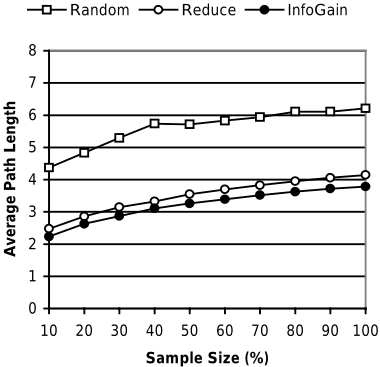
Average path lengths over 10 repeated trials for each sample size are shown in Figure 2. The results for Gini are not shown because they differ only slightly from those for InfoGain. While InfoGain performed slightly better than Gini for all sample sizes, its reduction in average path length relative to Gini was never more than one per cent. On the other hand, the Reduce criterion can be seen to provide a considerable reduction in average path length compared with selecting attributes purely at random. The additional reduction provided by InfoGain, though relatively small, is consistent over the range of sample sizes. While the average path length of the InfoGain trees increases as sample size increases, their efficiency is apparent even for the 100 per cent sample.
4.2 Which Criterion is Best for Binary Attributes?
Our second experiment compares the performance of InfoGain and Gini on irreducible data sets in which all attributes are binary. As noted in Section 3, Gini is equivalent in such data sets to the Reduce criterion. The data sets used in this experiment are randomly generated subsets of a complete, irreducible data set with 12 binary attributes. The class attribute is an integer that uniquely identifies each of the 4096 instances in the data set. Average path lengths for InfoGain and Gini over 10 repeated trials are shown in Figure 3 for subsets of the complete data set ranging in size from 10 to 100 per cent.
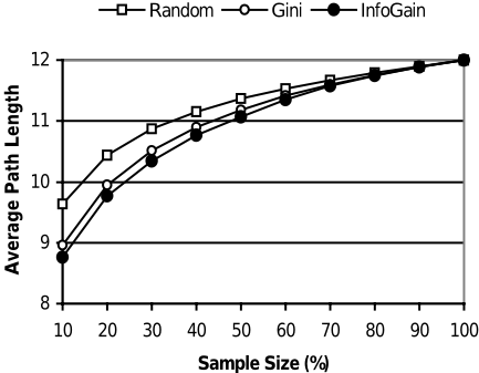
The effectiveness of both splitting criteria can be seen to decrease as sample size increases, with little reduction in average path length for sample sizes greater than 70 per cent. As predicted by our theoretical results, there is no reduction in average path length for the 100 per cent sample. However, for sample sizes less than 70 per cent, InfoGain now gives a noticeable improvement in comparison with Gini. The ability of Gini to almost match the performance of InfoGain on subsets of the AutoMPG data set may therefore be attributable to the absence of binary attributes in the data set.
4.3 How Close to Optimal is InfoGain?
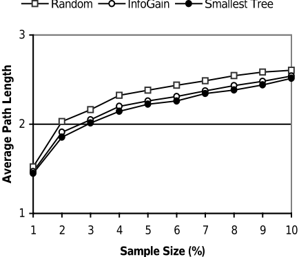
We can attempt to answer this question only for data sets in which the number of attributes is small enough for optimal trees to be identified by exhaustive search. The data sets in our third experiment are randomly generated subsets of a complete, irreducible data set in which each of 3 attributes has 10 values. By Proposition 2, the number of possible trees for any such data set is at most 3,072.
Figure 4 compares the average path length of InfoGain trees and optimal trees for subsets ranging in size from 1 to 10 per cent of the complete 10 × 10 × 10 data set. Based on averages over ten repeated trials, the results show that the InfoGain trees are close to optimal. Of the 100 InfoGain trees constructed in the experiment, 30 were optimal.
5 Related Work
Doyle and Cunningham [2000] applied a clustering algorithm to product data before using InfoGain to construct a decision tree. As shown by our results, however, InfoGain is often very effective in reducing average path length when applied directly to irreducible data sets. Doyle and Cunningham used a demand-driven or lazy approach to decision-tree induction, adapted from [Smyth and Cunningham, 1994], in which an explicit decision tree is not constructed. Instead, the user's answers are used to construct a single decision path. One advantage is that the user can select the attribute they consider most important instead of the one considered most useful by the system. In fault diagnosis, another advantage of a demand-driven approach to decision-tree induction is the system's ability to select the next most useful attribute to partition the case library when the user is unable to answer the most useful question [McSherry, 2001]. A demand-driven approach to the construction of identification trees is expected to provide similar benefits in a future version of Identify. The effects of incomplete data on retrieval performance, however, remain to be investigated.
Aha and Breslow [1997] used decision trees as an intermediate representation to improve the quality of conversational case libraries. In conversational CBR, the problem of irreducibility addressed in this paper is often complicated by the use of different features to describe cases. In fault diagnosis, for example, certain attributes may not be relevant or even meaningful for every case. The result is a high frequency of unanswered questions, or missing values, in cases. The splitting criterion used by Aha and Breslow to address this problem selected the attribute with fewest missing values. In the absence of missing values, though, this criterion is at best equivalent to selecting any attribute that is capable of splitting the data set and therefore inferior to InfoGain as shown by our results. In this paper, we have assumed the absence of missing values to simplify our initial comparison of splitting criteria for irreducible data sets. However, the impact of missing values on retrieval performance is an important issue to be addressed by further research.
Algorithms for building decision trees are usually evaluated by dividing a data set into a training set that is used to build a decision tree and a test set that is used to assess its predictive accuracy [Breslow and Aha, 1997].
However, an identification tree has no predictive accuracy; that is, it can correctly identify only the instances from which it was constructed. Evaluation in terms of predictive accuracy is equally compromised by irreducibility in the case library in CBR systems that rely on similarity-based retrieval. Aha et al. [1998] propose a leave-one-in approach to evaluating retrieval precision for conversational case libraries in which most (or all) cases have unique solutions. In their approach, each case is used as a test case but without removing it from the case library during testing. Precision is measured by how often the solution for the most similar case matches the solution for the test case. We plan to use a similar approach to the evaluation of precision in an investigation of the effects of incomplete data and missing values on retrieval performance in interactive CBR.
6 Conclusions
Minimizing the number of questions required to identify a fault, or a product that meets the requirements of the user, is an important objective in interactive CBR applications such as fault diagnosis, help-desk support, and on-line decision guides. Often in these applications, each case has a unique solution or represents a unique product in the case library. We have examined the performance of common splitting criteria for building identification trees to guide the retrieval of cases from such irreducible case libraries.
Our results show that the InfoGain criterion [Quinlan, 1986] is often more effective than other splitting criteria in reducing average path length when used to build identification trees from irreducible data sets. While the Gini criterion [Breiman et al., 1984] appears to compete well with InfoGain for attributes with several values, our results suggest that InfoGain may be more effective for binary attributes. The effectiveness of both criteria decreases as a data set (or case library) approaches completeness, and no reduction in average path length is possible in an irreducible data set that is also complete.
We have shown that for irreducible data sets, InfoGain and Gini can be expressed in terms of the frequencies of an attribute's values, thus providing a reduction in computational effort that may be of particular benefit in online decision guides. Issues to be addressed by further research include the effectiveness of techniques for tolerating missing values in decision tree learning [Quinlan, 1989] in the special case of identification trees.
References
- [Aha, 1998] David Aha. The omnipresence of case-based reasoning in science and application. Knowledge-Based Systems, 11:261-273, 1998.
- [Aha and Breslow, 1997] David Aha and Leonard Breslow. Refining conversational case libraries. In Proceedings of the Second International Conference on Case-Based Reasoning, pages 267-278, Providence, Rhode Island, 1997. Springer-Verlag.
- [Aha et al., 1998] David Aha, Tucker Maney and Leonard Breslow. Supporting dialogue inferencing in conversational case-based reasoning. In Proceedings of the Fourth European Workshop on Case-Based Reasoning, pages 262-273, Dublin, Ireland, 1998. Springer-Verlag.
- [Bergmann et al., 1999] Ralph Bergmann, Sean Breen, Mehmet Göker, Michael Manago and Stefan Wess. Developing Industrial Case-Based Reasoning Applications: The INRECA Methodology. SpringerVerlag, Berlin Heidelberg, 1999.
- [Blake and Merz, 1998] Catherine Blake and Christopher Merz. UCI Repository of Machine Learning Databases. University of California, Irving, California, 1998.
- [Breiman et al., 1984] Leo Breiman, Jerome Friedman, Richard Olshen and Charles Stone. Classification and Regression Trees. Wadsworth, Belmont, California, 1984.
- [Breslow and Aha, 1997] Leonard Breslow and David Aha. Simplifying decision trees: a survey. Knowledge Engineering Review, 12:1-40, 1997.
- [Cendrowska, 1987] Jadzia Cendrowska. PRISM: an algorithm for inducing modular rules. International Journal of Man-Machine Studies, 27:349-370, 1987.
- [Doyle and Cunningham, 2000] Michelle Doyle and Pádraig Cunningham. A dynamic approach to reducing dialog in on-line decision guides. In Proceedings of the Fifth European Workshop on Case-Based Reasoning, pages 49-60, Trento, 2000. Springer-Verlag.
- [McSherry, 2001] David McSherry. Interactive case-based reasoning in sequential diagnosis. Applied Intelligence, 14:65-76, 2001.
- [Quinlan, 1986] Ross Quinlan. Induction of decision trees. Machine Learning, 1:81-106, 1986.
- [Quinlan, 1989] Ross Quinlan. Unknown attribute values in induction. In Proceedings of the Sixth International Workshop on Machine Learning, pages 164-168, Ithaca, New York, 1989. Morgan Kaufmann.
- [Quinlan, 1993] Ross Quinlan. C4.5: Programs for Machine Learning. Morgan Kaufmann, San Mateo, California, 1993.
- [Smyth and Cunningham, 1994] Barry Smyth and Pádraig Cunningham. A comparison of incremental case-based reasoning and inductive learning. In Proceedings of the Second European Workshop on Case-Based Reasoning, pages 151-164, Chantilly, November 1994. SpringerVerlag.
- [Watson, 1997] Ian Watson. Applying Case-Based Reasoning: Techniques for Enterprise Systems. Morgan Kaufmann, San Francisco, California, 1997.
SiN: Integrating Case -based Reasoning with Task Decomposition
Héctor Muñoz-Avila, 1 David W. Aha, 2 Dana S. Nau, 1 Rosina Weber, 2 Len Breslow 2 & Fusun Yamal 1
1 Department of Computer Science, University of Maryland, College Park, MD 20742-3255
2 Navy Center for Applied Research in Artificial Intelligence, Naval Research Laboratory (Code 5515), Washington, DC 20375 1 lastname@cs.umd.edu 2 lastname@aic.nrl.navy.mil
Abstract
This paper describes SiN, a novel case-based planning algorithm that combines conversational case retrieval with generative planning. SiN is provably correct, and can generate plans given an incomplete domain theory by using cases to extend that domain theory. SiN can also reason with imperfect world-state information by incorporing preferences into the cases. Our empirical validation shows how these preferences affect plan quality.
1 Introduction
Generative planners traditionally require a complete domain theory, which provides a clear semantics for the planner's inferencing mechanism. This allows a planner to be used in different domains. However, in many planning domains, developing a complete domain theory is infeasible.
In this paper we present a case-based planning algorithm called SiN (SHOP integrated with NaCoDAE), which integrates the SHOP generative planner [Nau et al., 1999] with NaCoDAE, a conversational case retriever [Breslow & Aha, 1997]. SiN is a provably correct algorithm that does not require a complete domain theory nor complete information about initial or intermediate world-states.
In addition to describing SiN, which has been implemented in HICAP [Muñoz-Avila et al., 1999], we present sufficient conditions to ensure its correctness, show how SiN represents preferences in cases to generate plans in the context of imperfect world state information, and describe an empirical analysis that demonstrates the impact of the preferences on plan quality.
In the following sections, we introduce some terminology, detail SiN, including theoretical results on its semantics with respect to incomplete domain theory, present SiN's empirical evaluation to show the role of preferences to handle incomplete world state information, and discuss the implications of these results.
2 Motivation
SiN's design was partly motivated by the following characteristics of military planning operations.
- Military operations are strongly hierarchical [Mitchell 1997; Muñoz-Avila et al., 1999]. Thus, we chose to represent plans using Hierarchical Task Networks (HTNs) [Erol et al., 1994].
- There is an incomplete domain theory, in the form of general guidelines (doctrine) and standard operating procedures (SOPs). However, neither doctrine nor SOPs can be used to derive detailed tactical plans, which often require knowledge about previous experiences. Thus, SiN uses SHOP to perform first-principles reasoning and NaCoDAE to employ previous experiences.
- Military planners do not have complete information about the current situation; part of the planning includes dynamic information gathering, typically to assess enemy capabilities and/or deployment. In SiN, NaCODAE is used to plan with an incomplete world state using preferences, which we define in Section 4.
3 Notation and definitions
An HTN is a set of tasks and their ordering relations, denoted as N=({t1,…,tm},<) (m≥0), where < is a binary relation expressing temporal constraints between tasks. Decomposable tasks are called compound, while nondecomposable tasks are called primitive.
A domain theory consists of methods and operators for generating plans. A method is an expression of the form M=(h,P,ST), where h (the method's head) is a compound task, P is a set of preconditions , and ST is the set of M's (children) subtasks. M is applicable to a task t, relative to a state S (a set of ground atoms), iff matches(h,t,S) (i.e., h and t have the same predicate and arity, and a consistent set of bindings È exists that maps variables to values such that all terms in h match their corresponding ground terms in t) and the preconditions P are satisfied in S (i.e., there exists a consistent extension of È, named È', such that ∀ p∈P {pÈ' ∈S}), in which case M(t,S)=ST È'.
An operator is an expression of the form O=(h,aL,dL), where h (the operator's head) is a primitive task, and aL and dL are the so-called add- and delete-lists. These lists define how the operator's application transforms the current state S: every element in the add-list is added to S and every element in the delete-list is removed from S. An operator O is applicable to a task t, relative to a state S, iff matches(h,t,S).
A planning problem is a triple (T,S,D), where T is a set of tasks, S is a state, and D is a domain theory. A plan is the collection of primitive tasks obtained by decomposing all compound tasks in a planning problem (T,S,D).
4 Cases in SiN
In many domains it is impossible to assume that a complete domain theory of the world is known. For example, this is true when planning for non-combatant evacuations (NEOs). However, a partial domain theory exists for NEOs, and it can be elicited from doctrine and standard operating procedures [DOD, 1997].
Reasoning about parts of the domain for which no domain theory is available is done through cases. A case C is an instance of a method, denoted by C=(h,P,ST,Q), where h, P, and ST are defined as for methods and Q is a set of <question,answer> pairs. Q defines preferences for matching a case to the current state. Preferences are useful for ranking cases in the context of incomplete world states and/or domain theories because, as we will show, they focus users on providing relevant additional state information.
5 SiN mixed-initiative planner
SiN integrates SHOP and NaCoDAE's task decomposition algorithms. A single (current) state S is maintained in SiN that is accessible to and updateable by both SHOP and NaCoDAE. Answers given by the user during an interaction with NaCoDAE are added to S (i.e., each question has a translation into a ground atom). Changes to the state that occur by applying SHOP's operators are also reflected in S.
SHOP generative planner . At any point during the planning process, SHOP is refining a task list T' relative to a state S and a domain theory D. Initially, T' is the set of tasks T in the planning problem (T,S,D). SHOP performs ordered task decomposition [Nau et al., 2000], meaning that the tasks must be totally ordered (i.e., the < relation on HTNs is a total order). SHOP also maintains the partial solution plan p being derived (i.e., the primitive tasks in T'). Initially p is empty. SHOP selects the first task t in T' and continues as follows:
- If t is primitive and has an applicable operator O, then O is applied to t, S is updated accordingly, t is removed from T' and added to the end of p.
- Else if t is compound and has an applicable method M (that has not yet been applied to t), then M is applied, which replaces t in T' with M's subtasks.
- Else if T' is not empty, then SHOP backtracks.
- Else SHOP fails.
SHOP terminates when T' is empty, in which case p is the solution, or when SHOP tries to backtrack on a compound task t whose applicable methods have been exhausted.
NaCoDAE mixed -initiative case retriever . Users interact with NaCoDAE in conversations, which begin when the user selects a task t. NaCoDAE responds by displaying the top-ranked cases whose pre-conditions are satisfied and whose heads match t. Cases are ranked according to their similarity to the current state S, which is the state that exists at that time during the conversation. Similarity is computed for each case C by comparing the contents of S with Q, C's <q,a> preference pairs. (That is, each pair is represented as a monadic atom in S, and similarity for a given <q,a> preference pair becomes a membership test in S). NaCoDAE also displays questions, whose answers are not known in S, ranked according to their frequency among the top-ranked cases. The user can select and answer (with a) any displayed question q, which inserts <q,a> into S. This state change subsequently modifies the case and question rankings. A conversation ends when the user selects a case C, at which time the task t is decomposed into ST (i.e., C's subtasks).
SiN integrated planning a lgorithm . SiN receives as input a set of tasks T, a state, S, and a knowledge base I∪B consisting of an incomplete domain theory I and a collection of cases B. The output is a solution plan p consisting of a sequence of operators in I. Both SHOP and NaCoDAE assist SiN with refining T into a plan. As does SHOP, SiN maintains the set of tasks in T' that have not been decomposed and the partial solution plan p. At any point of time, either SHOP or NaCoDAE is in control and is focusing on a compound task t∈T' to decompose. SiN proceeds as follows:
- Rule # 1: If SHOP is in control and can decompose t, it does so and retains control. If SHOP cannot decompose t, but NaCoDAE has cases for decomposing t, then SHOP will cede control to NaCoDAE.
- Rule # 2: If NaCoDAE is in control, it has cases for decomposing t whose pre-conditions are satisfied. If the user applies one of them to decompose t, then NaCoDAE retains control. If NaCoDAE has no cases to decompose t or if the user decides not to apply any applicable case, then if t is SHOP-decomposable, NaCoDAE will cede control to SHOP.
If neither of these rules applies, then SiN backtracks, if possible. If backtracking is impossible (e.g., because t is a task in T), this planning process is interrupted and a failure is returned.
By continuing in this way, and assuming that the process is not interrupted with a failure, SiN will eventually yield a plan p (i.e., consisting only of primitive tasks).
6 Correctness of SiN
In this section we will assume that SiN performs ordered task decomposition. That is, we assume that all tasks are totally ordered and at each iteration, when refining a set of tasks T', SiN will start by decomposing the first task in T'. A relaxation of this condition should be possible once we modify SiN to include the extended version of SHOP that can represent partial-order task relations [Nau et al, 2001].
If I is an incomplete domain theory and B is a case base (i.e., a set of cases), then a domain theory D is consistent with I∪B iff (1) every method and operator in I is an instance of a method or operator in D and (2) for every case C=(h,P,ST,Q) in B, there is a method M=(h',P',ST') in D such that h, P, and ST are instances of h', P' and ST' respectively. Although many different domain theories might be consistent with I∪B, in general we will not know which of these is the one that produced I and B. However, we can prove that SiN is correct in the sense that, if it succeeds in outputting a plan, then that plan could have been generated by SHOP using any domain theory consistent with I∪B.
Proposition (Correctness of SiN) . Let T be a collection of tasks, S be an initial state, I be an incomplete domain theory, and B be a case base, and let SiN(T,S,I,B) represent the invocation of SiN with those items as inputs. Suppose that SiN performs ordered task decomposition. Then:
- If SiN(T,S,I,B) returns a plan p, then for every domain theory D consistent with I∪B, p is a solution plan for the planning problem (T,S,D).
- If SiN(T,S,I,B) cannot find a plan, then there is a domain theory D consistent with I∪B such that no solution plan exists for (T,S,D).
The proof is done by induction on the number of iterations of the SiN algorithm. The proof shows that each SiN task decomposition in (T,S,I∪B) corresponds to a SHOP task decomposition in (T,S,D). This is sufficient to prove correctness because SHOP is known to be correct [Nau et al., 1999]. We omit the details of the proof due to space limitations.
This proposition suggests that cases in SiN supply two kinds of knowledge: first, they provide control knowledge, similar to the knowledge encoded in cases using derivational replay when a complete domain theory is available [Veloso, 1994; Ihrig & Kambhampati, 1994]. Because cases are instances of methods, applying a case is comparable to a replay step in which the method selected to decompose a task is the one in the case's derivational trace. The main difference is that, while cases in replay systems correspond to a complete derivational trace, cases in SiN correspond to a single step in the derivational trace. Second, cases in SiN augment the domain theory and, thus, provide domain knowledge as do cases in many case-based planners (e.g., [Hammond, 1986]).
7 Imperfect World Information
SiN uses NaCoDAE to dynamically elicit the world state, which involves obtaining the user's preferences. Depending on the user's answers, cases will get re-ranked. When solving a task, the user can choose any of the cases, independent of their ranking, provided that all their preconditions are met. The preferences play a pivotal role in determining plan quality due to the absence of a complete domain theory.
Consider the following two simplified cases:
Case 1:
Head: selectTransport(ISB,NEOsite)
Preconditions: HelosAvailable(ISB)
Questions -Answer pai rs: Weather conditions? Fine
Subtasks: Transport(ISB,NEOsite,HELOS)
Case 2:
Head: selectTransport(ISB,NEOsite) Preconditions: groundTransportAvailable(ISB)
Questions -Answer pairs:
- Weather conditions? Rainy
- Imminent danger to evacuees? No
Subtasks: Transport(ISB,NEOsite,GroundTransport)
These cases both concern the selection of transportation means between an intermediate staging base (ISB) and the NEO site (NEOsite). The first case suggests using helicopters provided that they are available at the ISB. The second one suggests using ground transportation provided that the corresponding transportation means are available at the ISB. If the two cases are applicable, because both preconditions are met, the answers given by the user will determine a preference between them. For example if the weather is rainy and there is no immediate danger for the evacuees, NaCoDAE would suggest the second case. The rationale behind this is that flying in rainy conditions is risky. Thus, selecting ground transportation would be a better choice.
8 Evaluation
Our experiments focused on the role of preferences in the plan generation process in the context of incomplete world state information and how they affect the quality of the resulting plans. Towards this goal, we developed two planning domains where the contents of the world state can significantly impact choices during planning.
For these experiments, we encoded an automatic user that dynamically provided preferences when asked by NaCoDAE. The user provided preferences with a predefined bias (defined in the following sections) towards certain kinds of solutions. The automatic user will always select the case with the highest similarity. In situations where several candidate cases had the same highest similarity, the automatic user selected one of them randomly. The purpose was to observe whether the resulting plans reflect the user's bias despite the incomplete information about the world state.
8.1 The Personal Travel Domain
The first domain was the personal travel domain . Its plans concern traveling from locations in Washington, DC to downtown New York City (NYC). We encoded 7 transportation methods (3 inter- and 4 intra-city). Plans consist of 3-5 planning segments. States indicate different locations, whether connections between locations exists and by which means, weather conditions, etc. The knowledge base consists of 10 methods and 1 operator for SHOP and 40 cases for NaCoDAE.
Our personal travel plan evaluator can generate a different time duration each time it is given a plan and world state because of its non-deterministic execution. For each run, it outputs whether the plan succeeded and, if so, the trip's duration. A plan fails when segment delays cause a late arrival for a segment requiring a fixed time departure (e.g., an airplane flight). For each segment, we applied a delay function that is influenced by world state conditions. For example, a flight segment will incur a longer delay for higher chances of large snow accumulation, especially on holidays (i.e., high travel days). Segments are categorized into short, medium, and long lengths, and delays can range from 0 up to 4.5 times a segment's anticipated duration. Smaller multiples are used for maximum delays for medium (3.5) and long (2.5) duration segments.
We selected ten goals, corresponding to ten pairs of departing and arrival locations in Washington, DC and downtown NYC, respectively. For each goal, we generated 10 random world states, thus yielding 100 total planning problems. SiN was then used to generate a plan for each problem, thus yielding 300 plans. Each was executed 10 times by the plan evaluator, for a total of 3000 runs.
| Preference | Duration | Price | Success |
| Bus | 676 | 85 | 92.2% |
| Train | 466 | 176 | 94.3% |
| Plane | 375 | 338 | 77.0% |
Table 1 summarizes the results. When the user's bias was given towards taking the Bus for the intercity part of the trip. This preference yields maximal (676 minutes) durations, but has the cheapest price. On the other extreme, when the Plane is the preferred means of transportation, the duration is the shortest but the price is the most expensive. The lowest success rate occurs for plane trips; it reflects missing connections due to external factors such as the weather. Although a bias expresses a preference for a certain transportation mode, it does not imply that it was always selected; world state conditions may prevent the use of some travel modes for particular situations.
8.2 The NEO Planni ng Domain
The second domain was the Noncombatant Evacuation Operations Domain. Its plans involve performing a rescue mission where troops are grouped and transported between an initial location (the assembly point) and the NEO site (where the evacuees are located). After the troops arrived at the NEO site, evacuees are re-located to a safe haven. Planning involves selecting possible pre-defined routes, consisting of 4 segments each. The planner must also choose a transportation mode for each segment. In addition, other conditions were determined during planning such as whether communication exists with State Department personnel and the type of evacuee registration process. SiN's knowledge base included 6 operators, 22 methods, and 51 cases.
As with the personal travel domain evaluator, the NEO planning evaluator can generate a different output each time it is given a plan and a world state because of its nondeterministic execution. For each run, it outputs the plan execution duration, the time it took to reach the evacuees, and the evacuee casualties. Similar to the personal travel domain, we applied a delay function that is influenced by world state conditions. The Neo Planning evaluator is more complex than the personal travel evaluator because there are more conditions that can affect the output variables and these conditions may interact. For example, a small-sized force will incur fewer delays because embarking troops in the transportation means will take less time than for largesized forces. However, smaller force increase the chances of hostile attacks, which if they occur will delay the operation.
We had a single task, to perform a NEO, and generated 100 random world states, thus yielding 100 planning problems. SiN was then used to generate a plan for each problem, thus yielding 200 plans, and each was executed 10 times by the plan evaluator for a total of 2000 runs.
| Preference | Duration | Time to Reach Evacuees | Evacuee Casualties |
| Helicopter | 38.5 | 28.7 | 11% |
| Ground Vehicle | 48.1 | 34.8 | 16% |
Table 2 summarizes the results. The helicopter transport preference yields plans that have shorter execution durations (38.5 hours) and require less time to reach the evacuees (28.7 hours). In addition, average casualties among evacuees is less (11%), due mainly to the shorter time to reach them, and land travel is generally riskier than air travel. Still the number of casualties among evacuees is high even with helicopters. This is due to the simple bias encoded in the simulated user. Human users could yield better (and worse) plans by dynamically providing more sophisticated preferences depending on the world state conditions.
8.3 Discussion
The experiments show the capabilities of SiN in allowing the user to guide the planning process towards their preferences while dynamically capturing world-state conditions. Despite our use of simplistic simulated users, the quality of the plans reflect the user's bias.
9 Related Work
Table 3 compares seven different features of SiN to those of other planning systems.
| System | Gen | CBP | M-I | I | DK | CK |
|---|---|---|---|---|---|---|
| SiN | √ | √ √ | √ | √ | √ | √ |
| CHEF MI-CBP | √ | √ | √ | √ | √ | |
| NaCoDAE Prodigy/ | √ | √ √ | √ | √ | √ | |
| Analogy SHOP | √ | |||||
| SIPE II | √ | √ |
We first discuss the features shown in columns 2-5 of Table 3. SHOP [Nau et al., 1999], as is typical of generative planners, requires a complete domain theory. CHEF [Hammond, 1989] and DIAL [Leake et al., 1997] are case-based, but do not have a generative component, and thus need a large case base to perform well across a wide variety of problems. Prodigy/Analogy [Veloso, 1994], DerSNLP [Ihrig & Kambhampati, 1994], and Paris [Bergmann & Wilke, 1995] integrate generative and casebased planning, but require a complete domain theory and are not mixed-initiative. SIPE II [Wilkins, 1998] is a mixedinitiative generative planner, but does not use cases. NaCoDAE [Muñoz-Avila et al., 1999] is a mixed-initiative case-based planner, but does not employ generative planning.
At least three other integrated (case-based/generative), mixed-initiative planners exist. MI-CBP [Veloso et al., 1997], which extends Prodigy/Analogy, limits interaction to providing it with user feedback on completed plans. Thus, it must input, or learn thru feedback, a sufficiently complete domain theory to solve problems. In contrast, SiN gathers information it requires from the user through NaCoDAE conversations, but does not learn from user feedback. CAPlan/CbC [Muñoz-Avila et al., 1997] and Mitchell's
[1997] system use interaction for plan adaptation rather than to acquire state information.
Among integrated case-based/generative planners, SiN's interleaved control structure is unique in that it allows both subsystems to equally control the task decomposition process. In contrast, other approaches either use heuristics (Prodigy/Analogy; MI-CBP) or order case-based prior to generative planning [DerSNLP; Mitchell, 1997], although Paris does this iteratively through multiple abstraction levels. Distinguishing the relative advantages of these control strategies is an open research issue.
The final two columns of Table 3 refer to the types of contributions made by cases in CBP systems. CHEF and NaCoDAE both use cases to provide domain knowledge, while Prodigy/Analogy uses cases for control knowledge (i.e., determining which planning constructs to apply). In contrast, SiN uses cases to both provide domain knowledge (i.e., instances of methods) and control knowledge (i.e., it allows the user selects which of these instance methods to apply).
CaseAdvisor [Carrick et al., 1999], like SiN, integrates conversational case retrieval with planning. While CaseAdvisor applies pre-stored hierarchical plans to gather information to solve diagnosis tasks, SiN instead uses its case retriever to gather information and applies cases to refine hierarchical plans.
Planning with incomplete information has been the subject of frequent research in planning (e.g., [Golden et al., 1996]). Typically, a distinction between sensing and planning actions is made, where the former involve queries to external information sources and the latter involves inferencing steps. This is comparable to querying using NaCoDAE and task refinement using SHOP.
10 Final Remarks
We presented the SiN algorithm for case-based HTN planning. SiN was motivated by three requirements for planning military operations: plans are hierarchical, there is no complete domain theory explaining all possible courses of action, and planners do not have complete information about the current situation.
Our work includes the following contributions:
- SIN is a provably correct algorithm for case-based planning with incomplete domain theories.
- SiN can tolerate incomplete world state information by representing preferences in the cases. Our experimental results show that a user can dynamically guide SiN by giving preferences to it as part of the user's normal interaction with SiN during the planning process.
- SiN provides a bridge between two classical approaches for case-based planning, in which cases either provide control knowledge or domain knowledge. In SiN, cases provide both kinds of knowledge.
- SiN's ability to combine both experiential and generative knowledge sources can be beneficial in realworld domains where some processes are well known and others are obscure but recorded memories exists on how they were performed. Planning for NEOs is a typical example of this type of domain. We have integrated SiN into HICAP [Muñoz-Avila et al., 1999], a system designed to support these kinds of operations.
Our creation of SiN was made possible because of the similarity between NaCoDAE's cases and SHOP's methods. For our future work, we want to further exploit this similarity to ease knowledge acquisition for plan generation. To this end, we have started working to create algorithms for learning HTN methods automatically from cases.
Acknowledgements
The authors would like to thank the reviewers for their helpful comments. This research was supported by funding from DARPA, ONR, AFRL (F306029910013 and F3060200-2-0505), ARL (DAAL0197K0135), and the University of Maryland General Research Board. Opinions on SiN expressed in this paper are those of the authors and do not necessarily reflect the opinions of the funding agencies.
@inproceedings{ijcai2001p135,
  title     = {Minimizing Dialog Length in Interactive Case-Based Reasoning},
  author    = {McSherry, David},
  booktitle = {Proceedings of the Seventeenth International Joint Conference on
               Artificial Intelligence, {IJCAI-01}},
  publisher = {International Joint Conferences on Artificial Intelligence},
  editor    = {Bernhard Nebel},
  pages     = {993--997},
  year      = {2001},
  url       = {https://ijcai.org/proceedings/2001/135},
}
TY - CPAPER TI - Minimizing Dialog Length in Interactive Case-Based Reasoning AU - McSherry, David T2 - Proceedings of the Seventeenth International Joint Conference on Artificial Intelligence, IJCAI-01 PB - International Joint Conferences on Artificial Intelligence PY - 2001 SP - 993 EP - 997 UR - https://ijcai.org/proceedings/2001/135 ER -Copied
Machine-readable versions of this paper, for tools and AI agents:





