
The Foundations of Cost-Sensitive Learning
Proceedings of the Seventeenth International Joint Conference on Artificial Intelligence. Pages 973-977.
© 2001 International Joint Conferences on Artificial Intelligence
Abstract
This paper revisits the problem of optimal learning and decision-making when different misclassification errors incur different penalties. We characterize precisely but intuitively when a cost matrix is reasonable, and we show how to avoid the mistake of defining a cost matrix that is economically incoherent. For the two-class case, we prove a theorem that shows how to change the proportion of negative examples in a training set in order to make optimal cost-sensitive classification decisions using a classifier learned by a standard non-costsensitive learning method. However, we then argue that changing the balance of negative and positive training examples has little effect on the classifiers produced by standard Bayesian and decision tree learning methods. Accordingly, the recommended way of applying one of these methods in a domain with differing misclassification costs is to learn a classifier from the training set as given, and then to compute optimal decisions explicitly using the probability estimates given by the classifier.
- [Bauer and Kohavi, 1999] Eric Bauer and Ron Kohavi. An em- pirical comparison of voting classification algorithms: Bagging, boosting, and variants. Machine Learning, 36:105-139, 1999.
- [Bradford et al., 1998] J. Bradford, C. Kunz, R. Kohavi, C. Brunk, and C. Brodley. Pruning decision trees with misclassification costs. In Proceedings of the European Conference on Machine Learning, pages 131-136, 1998.
- [Breiman et al., 1984] L. Breiman, J. H. Friedman, R. A. Olshen, and C. J. Stone. Classification and Regression Trees. Wadswoth, Belmont, California, 1984.
- [Dietterich et al., 1996] T. G. Dietterich, M. Kearns, and Y. Man- sour. Applying the weak learning framework to understand and improve C4.5. In Proceedings of the Thirteenth International Conference on Machine Learning, pages 96-104.
- Morgan Kauf- mann, 1996.
- [Domingos and Pazzani, 1996] Pedro Domingos and Michael Paz- zani. Beyond independence: Conditions for the optimality of the simple Bayesian classifier. In Proceedings of the Thirteenth International Conference on Machine Learning, pages 105-112.
- Morgan Kaufmann, 1996.
- [Drummond and Holte, 2000] Chris Drummond and Robert C. Holte. Exploiting the cost (in)sensitivity of decision tree splitting criteria. In Proceedings of the Seventeenth International Confer- ence on Machine Learning, pages 239-246, 2000.
- [Japkowicz, 2000] N. Japkowicz. The class imbalance problem: Significance and strategies. In Proceedings of the International Conference on Artificial Intelligence, Las Vegas, June 2000.
- [Kearns and Mansour, 1996] M. Kearns and Y. Mansour. On the boosting ability of top-down decision tree learning algorithms. In Proceedings of the Annual ACM Symposium on the Theory of Computing, pages 459-468. ACM Press, 1996.
- [Kubat and Matwin, 1997] M. Kubat and S. Matwin. Addressing the curse of imbalanced training sets: One-sided sampling. In Proceedings of the Fourteenth International Conference on Ma- chine Learning, pages 179-186.
- Morgan Kaufmann, 1997.
- [Margineantu, 2000] Dragos Margineantu. On class probability es- timates and cost-sensitive evaluation of classifiers. In Workshop Notes, Workshop on Cost-Sensitive Learning, International Con- ference on Machine Learning, June 2000.
- [Michie et al., 1994] D. Michie, D. J. Spiegelhalter, and C. C. Tay- lor. Machine Learning, Neural and Statistical Classification. El- lis Horwood, 1994.
- [Provost and Domingos, 2000] Foster Provost and Pedro Domin- gos. Well-trained PETs: Improving probability estimation trees. Technical Report CDER #00-04-IS, Stern School of Business, New York University, 2000.
- [Weiss and Provost, 2001] Gary M. Weiss and Foster Provost. The effect of class distribution on classifier learning. Technical Re- port ML-TR 43, Department of Computer Science, Rutgers Uni- versity, 2001.
- [Zadrozny and Elkan, 2001a] Bianca Zadrozny and Charles Elkan. Learning and making decisions when costs and probabilities are both unknown. Technical Report CS2001-0664, Department of Computer Science and Engineering, University of California, San Diego, January 2001.
- [Zadrozny and Elkan, 2001b] Bianca Zadrozny and Charles Elkan. Obtaining calibrated probability estimates from decision trees and naive Bayesian classifiers. In Proceedings of the Eighteenth International Conference on Machine Learning, 2001. To appear.
References were extracted automatically from the PDF and may contain errors.
Full text extracted automatically from the PDF; figures, tables and equations may differ. The PDF is the version of record.
1 Making decisions based on a cost matrix
Given a specification of costs for correct and incorrect predictions, an example should be predicted to have the class that leads to the lowest expected cost, where the expectation is computed using the conditional probability of each class given the example. Mathematically, let the a0 ✁ ✄ ✆ ✞ entry in a cost matrix ✠ be the cost of predicting class ✁ when the true class is ✆ . If ✁ ✡ ✆ then the prediction is correct, while if ✁ ✌ ✡ ✆ the prediction is incorrect. The optimal prediction for an example ✏ is the class ✁ that minimizes
Costs are not necessarily monetary. A cost can also be a waste of time, or the severity of an illness, for example.
For each ✁ , ✑ a0 ✏ ✄ ✁ ✞ is a sumover the alternative possibilities for the true class of ✏ . In this framework, the role of a learning algorithm is to produce a classifier that for any example ✏ can estimate the probability ✙ a0 ✆ ✢ ✏ ✞ of each class ✆ being the true class of ✏ . For an example ✏ , making the prediction ✁ means acting as if ✁ is the true class of ✏ . The essence of cost-sensitive decision-making is that it can be optimal to act as if one class is true even when some other class is more probable. For example, it can be rational not to approve a large credit card transaction even if the transaction is most likely legitimate.
1.1 Cost matrix properties
A cost matrix ✠ always has the following structure when there are only two classes:
| actual negative | actual positive | |
|---|---|---|
| predict negative | ✠ a0 ✩ ✄ ✩ ✞ ✡ ✭ ✯ ✯ | ✠ a0 ✩ ✄ ✱ ✞ ✡ ✭ ✯ ✵ |
| predict positive | ✠ a0 ✱ ✄ ✩ ✞ ✡ ✭ ✵ ✯ | ✠ a0 ✱ ✄ ✱ ✞ ✡ ✭ ✵ ✵ |
Recent papers have followed the convention that cost matrix rows correspond to alternative predicted classes, while columns correspond to actual classes, i.e. row/column = ✁ / ✆ = predicted/actual.
In our notation, the cost of a false positive is ✭ ✵ ✯ while the cost of a false negative is ✭ ✯ ✵ . Conceptually, the cost of labeling an example incorrectly should always be greater than the cost of labeling it correctly. Mathematically, it should always be the case that ✭ ✵ ✯ ✹ ✭ ✯ ✯ and ✭ ✯ ✵ ✹ ✭ ✵ ✵ . We call these conditions the "reasonableness" conditions.
Suppose that the first reasonableness condition is violated, so ✭ ✯ ✯ ✼ ✭ ✵ ✯ but still ✭ ✯ ✵ ✹ ✭ ✵ ✵ . In this case the optimal policy is to label all examples positive. Similarly, if ✭ ✵ ✯ ✹ ✭ ✯ ✯ but ✭ ✵ ✵ ✼ ✭ ✯ ✵ then it is optimal to label all examples negative. We leave the case where both reasonableness conditions are violated for the reader to analyze.
Margineantu [2000] has pointed out that for some cost matrices, some class labels are never predicted by the optimal policy as given by Equation (1). We can state a simple, intuitive criterion for when this happens. Say that row ❂ dominates row ❃ in a cost matrix ✠ if for all ✆ , ✠ a0 ❂ ✄ ✆ ✞ ✼ ✠ a0 ❃ ✄ ✆ ✞ . In this case the cost of predicting ❃ is no greater than the cost of predicting ❂ , regardless of what the true class ✆ is. So it is optimal never to predict ❂ . As a special case, the optimal prediction is always ❃ if row ❃ is dominated by all other rows in a cost matrix. The two reasonableness conditions for a two-class cost matrix imply that neither row in the matrix dominates the other.
Given a cost matrix, the decisions that are optimal are unchanged if each entry in the matrix is multiplied by a positive constant. This scaling corresponds to changing the unit of account for costs. Similarly, the decisions that are optimal are unchanged ❇ if a constant is added to each entry in the matrix. This shifting corresponds to changing the baseline away from which costs are measured. By scaling and shifting entries, any two-class cost matrix that satisfies the reasonableness conditions can be transformed into a simpler matrix that always leads to the same decisions:
where ✭ ❈ ✯ ✵ ✡ a0 ✭ ✯ ✵ ❋ ✭ ✯ ✯ ✞ ❍ a0 ✭ ✵ ✯ ❋ ✭ ✯ ✯ ✞ and ✭ ❈ ✵ ✵ ✡ a0 ✭ ✵ ✵ ❋ ✭ ✯ ✯ ✞ ❍ a0 ✭ ✵ ✯ ❋ ✭ ✯ ✯ ✞ . Fromamatrix perspective, a 2x2 cost matrix effectively has two degrees of freedom.
1.2 Costs versus benefits
Although most recent research in machine learning has used the terminology of costs, doing accounting in terms of benefits is generally preferable, because avoiding mistakes is easier, since there is a natural baseline from which to measure all benefits, whether positive or negative. This baseline is the state of the agent before it takes a decision regarding an example. After the agent has made the decision, if it is better off, its benefit is positive. Otherwise, its benefit is negative.
When thinking in terms of costs, it is easy to posit a cost matrix that is logically contradictory because not all entries in the matrix are measured from the same baseline. For example, consider the so-called German credit dataset that was published as part of the Statlog project [Michie et al., 1994]. The cost matrix given with this dataset is as follows:
| actual bad | actual good | |
|---|---|---|
| predict bad | 0 | 1 |
| predict good | 5 | 0 |
Here examples are people who apply for a loan from a bank. "Actual good" means that a customer would repay a loan while "actual bad" means that the customer would default. The action associated with "predict bad" is to deny the loan. Hence, the cashflow relative to any baseline associated with this prediction is the same regardless of whether "actual good" or "actual bad" is true. In every economically reasonable cost matrix for this domain, both entries in the "predict bad" rowmust be the same.
Costs or benefits can be measured against any baseline, but the baseline must be fixed. An opportunity cost is a foregone benefit, i.e. a missed opportunity rather than an actual penalty. It is easy to make the mistake of measuring different opportunity costs against different baselines. For example, the erroneous cost matrix above can be justified informally as follows: "The cost of approving a good customer is zero, and the cost of rejecting a bad customer is zero, because in both cases the correct decision has been made. If a good customer is rejected, the cost is an opportunity cost, the foregone profit of 1. If a bad customer is approved for a loan, the cost is the lost loan principal of 5."
To see concretely that the reasoning in quotes above is incorrect, suppose that the bank has one customer of each of the four types. Clearly the cost matrix above is intended to imply that the net change in the assets of the bank is then ❋ 4. Alternatively, suppose that we have four customers who receive loans and repay them. The net change in assets is then +4. Regardless of the baseline, any method of accounting should give a difference of 8 between these scenarios. But with the erroneous cost matrix above, the first scenario gives a total cost of 6, while the second scenario gives a total cost of 0.
In general the amount in some cells of a cost or benefit matrix may not be constant, and may be different for different examples. For example, consider the credit card transactions domain. Here the benefit matrix might be
| fraudulent | legitimate | |
|---|---|---|
| refuse | $20 | ❋ $20 |
| approve | ❋ ✏ | 0.02✏ |
where ✏ is the size of the transaction in dollars. Approving a fraudulent transaction costs the amount of the transaction because the bank is liable for the expenses of fraud. Refusing a legitimate transaction has a non-trivial cost because it annoys a customer. Refusing a fraudulent transaction has a nontrivial benefit because it may prevent further fraud and lead to the arrest of a criminal. Research on cost-sensitive learning and decision-making when costs may be example-dependent is only just beginning [Zadrozny and Elkan, 2001a].
1.3 Making optimal decisions
In the two-class case, the optimal prediction is class 1 if and only if the expected cost of this prediction is less than or equal to the expected cost of predicting class 0, i.e. if and only if
which is equivalent to
given ❘ ✡ ✙ a0 ✆ ✡ ✱ ✢ ✏ ✞ . If this inequality is in fact an equality, then predicting either class is optimal.
The threshold for making optimal decisions is ❘ ❱ such that
Assuming the reasonableness conditions the optimal prediction is class 1 if and only if ❘ ✼ ❘ ❱ . Rearranging the equation for ❘ ❱ leads to the solution
assuming the denominator is nonzero, which is implied by the reasonableness conditions. This formula for ❘ ❱ shows that any 2x2 cost matrix has essentially only one degree of freedom from a decision-making perspective, although it has two degrees of freedom from a matrix perspective. The cause of the apparent contradiction is that the optimal decision-making policy is a nonlinear function of the cost matrix.
2 Achieving cost-sensitivity by rebalancing
In this section we turn to the question of how to obtain a classifier that is useful for cost-sensitive decision-making.
Standard learning algorithms are designed to yield classifiers that maximize accuracy. In the two-class case, these classifiers implicitly make decisions based on the probability threshold 0.5. The conclusion of the previous section was that we need ❨ a classifier that given an example ✏ , says whether or not ✙ a0 ✆ ✡ ✱ ✢ ✏ ✞ ✼ ❘ ❱ for some target threshold ❘ ❱ that in general is different from 0.5. How can a standard learning algorithm be made to produce a classifier that makes decisions based on a general ❘ ❱ ?
The most common method of achieving this objective is to rebalance the training set given to the learning algorithm, i.e. to change the the proportion of positive and negative training examples in the training set. Although rebalancing is a common idea, the general formula for how to do it correctly has not been published. The following theorem provides this formula.
Theorem 1: To make a target probability threshold ❘ ❱ correspond to a given probability threshold ❘ ✯ , the number of negative examples in the training set should be multiplied by
While the formula in Theorem 1 is simple, the proof of its correctness is not. We defer the proof until the end of the next section.
In the special case where the threshold used by the learning method is ❘ ❭ ✡ ✩ ✥ ❴ and ✭ ✯ ✯ ✡ ✭ ✵ ✵ ✡ ✩ , the theorem says that the number of negative training examples should be multiplied by ❘ ❱ ❍ a0 ✱ ❋ ❘ ❱ ✞ ✡ ✭ ✵ ✯ ❍ ✭ ✯ ✵ ✥ This special case is used by Breiman et al. [1984].
The directionality of Theorem 1 is important to understand. Suppose we have a learning algorithm ✑ that yields classifiers that make predictions based on a probability threshold ❘ ✯ . Given a training set ❝ and a desired probability threshold ❘ ❱ , the theorem says how to create a training set ❝ ❈ by changing the number of negative training examples such that ✑ applied to ❝ ❈ gives the desired classifier.
Theorem 1 does not say in what way the number of negative examples should be changed. If a learning algorithm can use weights on training examples, then the weight of each negative example can be set to the factor given by the theorem. Otherwise, we must do oversampling or undersampling. Oversampling means duplicating examples, and undersampling means deleting examples.
Sampling can be done either randomly or deterministically. While deterministic sampling can reduce variance, it risks introducing bias, if the non-random choice of examples to duplicate or eliminate is correlated with some property of the examples. Undersampling that is deterministic in the sense that the fraction of examples with each value of a certain feature is held constant is often called stratified sampling.
It is possible to change the number of positive examples instead of or as well as changing the number of negative examples. However in many domains one class is rare compared to the other, and it is important to keep all available examples of the rare class. In these cases, if we call the rare class the positive class, Theorem 1 says directly how to change the number of common examples without discarding or duplicating any of the rare examples.
3 New probabilities given a new base rate
In this section we state and prove a theorem of independent interest that happens also to be the tool needed to prove Theorem 1. The new theorem answers the question of how the predicted class membership probability of an example should change in response to a change in base rates. Suppose that ❘ ✡ ✙ a0 ✆ ✡ ✱ ✢ ✏ ✞ is correct for an example ✏ , if ✏ is drawn from a population with base rate ❡ ✡ ✙ a0 ✆ ✡ ✱ ✞ positive examples. But suppose that in fact ✏ is drawn from a population with base rate ❡ ❈ . What is ❘ ❈ ✡ ✙ ❈ a0 ✆ ✡ ✱ ✢ ✏ ✞ ?
We make the assumption that the shift in base rate is the only change in the population to which ✏ belongs. Formally, we assume that within the positive and negative subpopulations, example probabilities are unchanged: ✙ ❈ a0 ✏ ✢ ✆ ✡ ✱ ✞ ✡ ✙ a0 ✏ ✢ ✆ ✡ ✱ ✞ and ✙ ❈ a0 ✏ ✢ ✆ ✡ ✩ ✞ ✡ ✙ a0 ✏ ✢ ✆ ✡ ✩ ✞ . Given these assumptions, the following theorem shows how to compute ❘ ❈ as a function of ❘ , ❡ , and ❡ ❈ .
Theorem 2: In the context just described,
Proof: Using Bayes' rule, ❘ ✡ ✙ a0 ✆ ✡ ✱ ✢ ✏ ✞ is
Because ✆ ✡ ✱ and ✆ ✡ ✩ are mutually exclusive, ✙ a0 ✏ ✞ is
Let ✭ ✡ ✙ a0 ✏ ✢ ✆ ✡ ✱ ✞ , let ♦ ✡ ✙ a0 ✏ ✢ ✆ ✡ ✩ ✞ , and let ♣ ✡ ♦ ❍ ✭ . Then
Similarly,
Now we can solve for ♣ as a function of ❘ and ❡ . We have ❘ ❡ ▲ ❘ ♣ a0 ✱ ❋ ❡ ✞ ✡ ❡ so ♣ ✡ a0 ❡ ❋ ❘ ❡ ✞ ❍ a0 ❘ ❋ ❘ ❡ ✞ ✥ Then the denominator for ❘ ❈ is
Finally we have
It is important to note that Theorem 2 is a statement about true probabilities given different base rates. The proof does not rely on how probabilities may be estimated based on some learning process. In particular, the proof does not use any assumptions of independence or conditional independence, as made for example by a naive Bayesian classifier.
If a classifier yields estimated probabilities ✈ ❘ that we assume are correct given a base rate ❡ , then Theorem 2 lets us
0
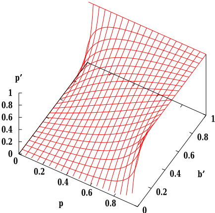
Figure 1: ❘ ❈ as a function of ❘ and ❡ , when ❡ ❈ ✡ ✩ ✥ ❴ .
compute estimated probabilities ✈ ❘ ❈ that are correct given a different base rate ❡ ❈ . From this point of view, the theorem has a remarkable aspect. It lets us use a classifier learned from a training set drawn from one probability distribution on a test set drawn from a different probability distribution. The theorem thus relaxes one of the most fundamental assumptions of almost all research on machine learning, that training and test sets are drawn from the same population.
The insight in the proof is the introduction of the variable ♣ that is the ratio of ✙ a0 ✏ ✢ ✆ ✡ ✩ ✞ and ✙ a0 ✏ ✢ ✆ ✡ ✱ ✞ . If we try to compute the actual values of these probabilities, we find that we have more variables to solve for than we have simultaneous equations. Fortunately, all we need to know for any particular example ✏ is the ratio ♣ .
The special case of Theorem 2 where ❘ ❈ ✡ ✩ ✥ ❴ was recently worked out independently by Weiss and Provost [2001]. The case where ❡ ✡ ✩ ✥ ❴ is also interesting. Suppose that we do not know the base rate of positive examples at the time we learn a classifier. Then it is reasonable to use a training set with ❡ ✡ ✩ ✥ ❴ . Theorem 2 says how to compute probabilities ❘ ❈ later that are correct given that the population of test examples has base rate ❡ ❈ . Specifically,
This function of ❘ and ❡ ❈ is plotted in Figure 1.
Using Theorem 2 as a lemma, we can now prove Theorem 1 with a slight change of notation.
Theorem 1: To make a target probability threshold ❘ correspond to a given probability threshold ❘ ❈ , the number of negative training examples should be multiplied by
Proof: We want to compute an adjusted base rate ❡ ❈ such that for a classifier trained using this base rate, an estimated probability ❘ ❈ corresponds to a probability ❘ for a classifier trained using the base rate ❡ .
We need to compute the adjusted ❡ ❈ as a function of ❡ , ❘ , and ❘ ❈ . From the proof of Theorem 2, ❘ ❈ ❡ ❋ ❘ ❈ ❘ ❡ ▲ ❘ ❈ ❡ ❈ ❘ ❋ ❘ ❈ ❡ ❡ ❈ ✡ ❡ ❈ ❘ ❋ ❡ ❈ ❘ ❡ . Collecting all the ❡ ❈ terms on the left, we have ❡ ❈ ❘ ❋ ❡ ❈ ❘ ❡ ❋ ❡ ❈ ❘ ❈ ❘ ▲ ❡ ❈ ❘ ❈ ❡ ✡ ❘ ❈ ❡ ❋ ❘ ❈ ❘ ❡ , which gives that the adjusted base rate should be
Suppose that ❡ ✡ ✱ ❍ a0 ✱ ▲ ❃ ✞ and ❡ ❈ ✡ ✱ ❍ a0 ✱ ▲ ❃ ❈ ✞ so the number of negative training examples should be multiplied by ❃ ❈ ❍ ❃ to get the adjusted base rate ❡ ❈ . We have that ❃ ❈ ✡ a0 ✱ ❋ ❡ ❈ ✞ ❍ ❡ ❈ is
Therefore
Note that the effective cardinality of the subset of negative training examples must be changed in a way that does not change the distribution of examples within this subset.
4 Effects of changing base rates
Changing the training set prevalence of positive and negative examples is a common method of making a learning algorithm cost-sensitive. A natural question is what effect such a change has on the behavior of standard learning algorithms. Separately, many researchers have proposed duplicating or discarding examples when one class of examples is rare, on the assumption that standard learning methods perform better when the prevalence of different classes is approximately equal [Kubat and Matwin, 1997; Japkowicz, 2000]. The purpose of this section is to investigate this assumption.
4.1 Changing base rates and Bayesian learning
Given an example ✏ , a Bayesian classifier applies Bayes' rule to compute the probability of each class ✆ as ✙ a0 ✆ ✢ ✏ ✞ ✡ ✙ a0 ✏ ✢ ✆ ✞ ✙ a0 ✆ ✞ ❍ ✙ a0 ✏ ✞ ✥ Typically ✙ a0 ✏ ✢ ✆ ✞ is computed by a function learned froma training set, ✙ a0 ✆ ✞ is estimated as the training set frequency of class ✆ , and ✙ a0 ✏ ✞ is computed indirectly by solving the equation ❷ ✗ ✙ a0 ✆ ✢ ✏ ✞ ✡ ✱ .
A Bayesian learning method essentially learns a model ✙ a0 ✏ ✢ ✆ ✞ of each class ✆ separately. If the frequencyof a class is changed in the training set, the only change is to the estimated base rate ✙ a0 ✆ ✞ of each class. Therefore there is little reason to expect the accuracy of decision-making with a Bayesian classifier to be higher with any particular base rates.
Naive Bayesian classifiers are the most important special case of Bayesian classification. A naive Bayesian classifier is based on the assumption that within each class, the values of the attributes of examples are independent. It is well-known that these classifiers tend to give inaccurate probability estimates [Domingos and Pazzani, 1996]. Given an example ✏ , suppose that a naive Bayesian classifier computes ❸ ❹ a0 ✏ ✞ as its estimate of ✙ a0 ✆ ✡ ✱ ✢ ✏ ✞ . Usually ❹ a0 ✏ ✞ is too extreme: for most ✏ , either ❹ a0 ✏ ✞ is close to 0 and then ❹ a0 ✏ ✞ ❺ ✙ a0 ✆ ✡ ✱ ✢ ✏ ✞ or ❹ a0 ✏ ✞ is close to 1 and then ❹ a0 ✏ ✞ ✹ ✙ a0 ✆ ✡ ✱ ✢ ✏ ✞ .
However, the ranking of examples by naive Bayesian classifiers tends to be correct: if ❹ a0 ✏ ✞ ❺ ❹ a0 ❼ ✞ then ✙ a0 ✆ ✡ ✱ ✢ ✏ ✞ ❺ ✙ a0 ✆ ✡ ✱ ✢ ❼ ✞ . This fact suggests that given a costsensitive application where optimal decision-making uses the probability threshold ❘ ❱ , one should empirically determine a different threshold ❽ ❘ such that ❹ a0 ✏ ✞ ✼ ❽ ❘ is equivalent to ✙ a0 ✆ ✡ ✱ ✢ ✏ ✞ ✼ ❘ ❱ . This procedure is likely to improve the accuracy of decision-making, while changing the proportion of negative examples using Theorem 1 in order to use the threshold 0.5 is not.
4.2 Decision tree growing
We turn our attention now to standard decision tree learning methods, which have two phases. In the first phase a tree is grown top-down, while in the second phase nodes are pruned from the tree. We discuss separately the effect on each phase of changing the proportion of negative and positive training examples.
A splitting criterion is a metric applied to an attribute that measures how homogeneous the induced subsets are, if a training set is partitioned based on the values of this attribute. Consider a discrete attribute ➀ that has values ➀ ✡ ➁ ✵ through ➀ ✡ ➁ ➂ for some ❂ ✼ ③ . In the two-class case, standard splitting criteria have the form
where ❘ ➄ ✡ ✙ a0 ✆ ✡ ✱ ✢ ➀ ✡ ➁ ➄ ✞ and all probabilities are frequencies in the training set to be split based on ➀ . The function ➆ a0 ❘ ✄ ✱ ❋ ❘ ✞ measures the impurity or heterogeneity of each subset of training examples. All such functions are qualitatively similar, with a unique maximum at ❘ ✡ ✩ ✥ ❴ , and equal minima at ❘ ✡ ✩ and ❘ ✡ ✱ .
Drummond and Holte [2000] have shown that for twovalued attributes the impurity function ③ ➉ ❘ a0 ✱ ❋ ❘ ✞ suggested by Kearns and Mansour [1996] is invariant to changes in the proportion of different classes in the training data. We prove here a more general result that applies to all discretevalued attributes and that shows that related impurity functions, including the Gini index [Breiman et al., 1984], are not invariant to base rate changes.
Theorem 3: Suppose ➆ a0 ❘ ✄ ✱ ❋ ❘ ✞ ✡ ➋ a0 ❘ a0 ✱ ❋ ❘ ✞ ✞ ➍ where ➋ ✹ ✩ and ➎ ✹ ✩ . For any collection of discrete-valued attributes, the attribute that minimizes ➃ a0 ➀ ✞ using ➆ is the same regardless of changes in the base rate ✙ a0 ✆ ✡ ✱ ✞ of the training set if ➎ ✡ ✩ ✥ ❴ , and not otherwise in general.
Proof: For any attribute ➀ , by definition
where ➁ ✵ through ➁ ➂ are the possible values of ➀ . So by Bayes' rule ➃ a0 ➀ ✞ ❍ ➋ is
Grouping the ✙ a0 ➁ ➄ ✞ factors for each ➐ gives that ➃ a0 ➀ ✞ ❍ ➋ is
Now the base rate factors can be brought outside the sum, so ➃ a0 ➀ ✞ is ➋ ➑ ✵ ✙ a0 ✆ ✡ ✱ ✞ ➍ ✙ a0 ✆ ✡ ✩ ✞ ➍ times the sum
Because ➋ ➑ ✵ ✙ a0 ✆ ✡ ✱ ✞ ➍ ✙ a0 ✆ ✡ ✩ ✞ ➍ is constant for all attributes, the attribute ➀ for which ➃ a0 ➀ ✞ is minimum is determined by the minimum of (3). If ③ ➎ ✡ ✱ then (3) depends only on ✙ a0 ➁ ➄ ✢ ✆ ✡ ✱ ✞ and ✙ a0 ➁ ➄ ✢ ✆ ✡ ✩ ✞ , which do not depend on the base rates. Otherwise, (3) is different for different base rates because
unless the attribute ➀ is independent of the class ✆ , that is ✙ a0 ➁ ➄ ✢ ✆ ✡ ✱ ✞ ✡ ✙ a0 ➁ ➄ ✢ ✆ ✡ ✩ ✞ for ✱ a80 ➐ a80 ❂ .
The sum (3) has its maximum value 1 if ➀ is independent of ✆ . As desired, the sum is smaller otherwise, if ➀ and ✆ are correlated and hence splitting on ➀ is reasonable.
Theorem 3 implies that changing the proportion of positive or negative examples in the training set has no effect on the structure of the tree if the decision tree growing method uses the ③ ➉ ❘ a0 ✱ ❋ ❘ ✞ impurity criterion. If the algorithm uses a different criterion, such as the C4.5 entropy measure, the effect is usually small, because all impurity criteria are similar.
The experimental results of Drummond and Holte [2000] and Dietterich et al. [1996] show that the ③ ➉ ❘ a0 ✱ ❋ ❘ ✞ criterion normally leads to somewhat smaller unpruned decision trees, sometimes leads to more accurate trees, and never leads to much less accurate trees. Therefore we can recommend its use, and we can conclude that regardless of the impurity criterion, applying Theorem 1 is not likely to have have much influence on the growing phase of decision tree learning.
4.3 Decision tree pruning
Standard methods for pruning decision trees are highly sensitive to the prevalence of different classes among training examples. If all classes except one are rare, then C4.5 often prunes the decision tree down to a single node that classifies all examples as members of the common class. Such a classifier is useless for decision-making if failing to recognize an example in a rare class is an expensive error.
Several papers have examined recently the issue of how to obtain good probability estimates from decision trees [Bradford et al., 1998; Provost and Domingos, 2000; Zadrozny and Elkan, 2001b]. It is clear that it is necessary to use a smoothing method to adjust the probability estimates at each leaf of a decision tree. It is not so clear what pruning methods are best.
The experiments of Bauer and Kohavi [1999] suggest that no pruning is best when using a decision tree with probability smoothing. The overall conclusion of Bradford et al. [1998] is that ↔ the best pruning is either no pruning or what they call "Laplace pruning." The idea of Laplace pruning is:
- Do Laplace smoothing: If ❃ training examples reach a node, of which ➐ are positive, let the estimate at this node of ✙ a0 ✆ ✡ ✱ ✢ ✏ ✞ be a0 ➐ ▲ ✱ ✞ ❍ a0 ❃ ▲ ③ ✞ .
- Compute the expected loss at each node using the smoothed probability estimates, the cost matrix, and the training set.
- If the expected loss at a node is less than the sum of the expected losses at its children, prune the children.
We can show intuitively that Laplace pruning is similar to no pruning. In the absence of probability smoothing, the expected loss at a node is always greater than or equal to the sum of the expected losses at its children. Equality holds only if the optimal predicted class at each child is the same as the optimal predicted class at the parent. Therefore, in the absence of smoothing, step (3) cannot change the meaning of a decision tree, i.e. the classes predicted by the tree, so Laplace pruning is equivalent to no pruning.
With probability smoothing, if the expected loss at a node is less than the sum of the expected losses at its children, the difference must be caused by smoothing, so without smoothing there would presumably be equality. So pruning the children is still only a simplification that leaves the meaning of the tree unchanged. Note that the effect of Laplace smoothing is small at internal tree nodes, because at these nodes typically ➐ ✹ ✹ ✱ and ❃ ✹ ✹ ③ .
In summary, growing a decision tree can be done in a cost-insensitive way. When using a decision tree to estimate probabilities, it is preferable to do no pruning. If costs are example-dependent, then decisions should be made using smoothed probability estimates and Equation (1). If costs are fixed, i.e. there is a single well-defined cost matrix, then each node in the unpruned decision tree can be labeled with the optimal predicted class for that leaf. If all the leaves under a certain node are labeled with the same class, then the subtree under that node can be eliminated. This simplification makes the tree smaller but does not change its predictions.
5 Conclusions
This paper has reviewed the basic concepts behind optimal learning and decision-making when different misclassification errors cause different losses. For the two-class case, we have shown rigorously how to increase or decrease the proportion of negative examples in a training set in order to make optimal cost-sensitive classification decisions using a classifier learned by a standard non cost-sensitive learning method. However, we have investigated the behavior of Bayesian and decision tree learning methods, and concluded that changing the balance of negative and positive training examples has little effect on learned classifiers. Accordingly, the recommended way of using one of these methods in a domain with differing misclassification costs is to learn a classifier from the training set as given, and then to use Equation (1) or Equation (2) directly, after smoothing probability estimates and/or adjusting the threshold of Equation (2) empirically if necessary.
@inproceedings{ijcai2001p133,
  title     = {The Foundations of Cost-Sensitive Learning},
  author    = {Elkan, Charles},
  booktitle = {Proceedings of the Seventeenth International Joint Conference on
               Artificial Intelligence, {IJCAI-01}},
  publisher = {International Joint Conferences on Artificial Intelligence},
  editor    = {Bernhard Nebel},
  pages     = {973--977},
  year      = {2001},
  url       = {https://ijcai.org/proceedings/2001/133},
}
TY - CPAPER TI - The Foundations of Cost-Sensitive Learning AU - Elkan, Charles T2 - Proceedings of the Seventeenth International Joint Conference on Artificial Intelligence, IJCAI-01 PB - International Joint Conferences on Artificial Intelligence PY - 2001 SP - 973 EP - 977 UR - https://ijcai.org/proceedings/2001/133 ER -Copied
Machine-readable versions of this paper, for tools and AI agents:





