
A Divide and Conquer Bidirectional Search: First Results
Proceedings of the Sixteenth International Joint Conference on Artificial Intelligence. Search. Pages 1184-1190.
© 1999 International Joint Conferences on Artificial Intelligence
Abstract
We present a new algorithm to reduce the space complexity of heuristic search. It is most effective for problem spaces that grow polynomially with problem size, but contain large numbers of short cycles. For example, the problem of finding a lowest-cost corner-to-corner path in a d-dimensional grid has app li cation to gene sequence alignment in computational biology. Th e main id ea is to perform a bidirectional search, but saving only the Open lists and not the Closed lists. Once the search completes, we have one node on an optimal path, but don't have the solution path itself. The path is then reconstructed by recursively applying the same algo rithm between the initial node and the intermediate node, and also between the intermediate node and the goal node. If n is the length of the grid in each dimension, and d is the number of dimensions, this algor ithm reduces the memory requirement from O(nd) to O(nd-l ). Th e time complexity only increases by a constant factor of 1r in two dimensions, and 7rV3/3 ::::::: 1.8 in three dimensions.
- Carrillo, H., and D. Lipman, The multiple sequence alignment problem in biology, SIAM Journal of Ap- plied Mathematics, Vol. 48, No.5, October 1988, pp. 1073-1082.
- Dijkstra, E.W., A note on two problems in connex- ion with graphs, Numerische Mathematik, Vol. 1, 1959, pp. 269-71.
- Hirschberg, D.S., A linear space algorithm for com- puting maximal common subsequences, Communi- cations of the ACM, Vol. 18, No. 6, June, 1975, pp. 341-343.
- Hart, P.E., N.J. Nilsson, and B. Raphael, A formal basis for the heuristic determination of minimum cost paths, IEEE Transactions on Systems Science and Cybernetics, Vol. SSC-4, No. 2, July 1968, pp. 100-107.
- Ikeda, T., and H. Imai, Enhanced A* algorithms for multiple alignments: optimal alignments for sev- eral sequences and k-opt approximate alignments for large cases, Theoretical Computer Science, Vol. 210, 1998.
- Kernighan, B.W., and D.M. Ritchie, The C Pro- gramming Language, second edition, Prentice Hall, Englewood Cliffs, N.J., 1988.
- Korf, R.E., Space-efficient search algorithms, Com- puting Surveys, Vol. 27, No. 3, Sept., 1995, pp. 337- 339.
- Korf, R.E., Depth-first iterative-deepening: An op- timal admissible tree search, Artificial Intelligence, Vol. 27, No. 1, 1985, pp. 97-109.
- Korf, R.E., and D.M. Chickering, Best-first mini- max search, Artificial Intelligence, Vol. 84, No. 1-2, July 1996, pp. 299-337.
- Miura, T., and T. Ishida, Stochastic node caching for memory-bounded search, Proceedings of the Na- tional Conference on Artificial Intelligence { AAAI- 98), Madison, WI, July, 1998, pp. 450-456.
- Taylor, L., and R.E. Korf, Pruning duplicate nodes in depth-first search, Proceedings of the National Conference on Artificial Intelligence ( AAAI-93 ), Washington D.C., July 1993, pp. 756-761.
References were extracted automatically from the PDF and may contain errors.
Full text extracted automatically from the PDF; figures, tables and equations may differ. The PDF is the version of record.
1 Introduction
Consider an n x m grid, where each edge has a poten tially different cost associated with it. We want a lowest cost path from the upper-lefthand corner to the opposite lower-righthand corner, where the cost of a path is the sum of the costs of the edges in it. One important ap plication of this problem is finding the best alignment of two genes of lengths n and m, represented as sequences of amino acids [Carrillo and Lipman, 1988]. We omit the details of the mapping between these two problems, and present it only to suggest that the problem is of practical importance. If we want to align d different se quences simultaneously, the problem generalizes to find ing a lowest-cost path in a d-dimensional grid.
Another example of this problem is that of finding a shortest path in a maze. In this case, an edge between two nodes either has a finite cost, indicating that there is a direct path between the two nodes, or an infinite cost, indicating there is a wall between them.
In this paper, we consider only the orthogonal moves up, down, left and right, and want a lowest-cost path from one corner to another. The extension to include di agonal moves is straightforward. While our experiments use a two-dimensional grid, the algorithm trivially gen eralizes to multiple dimensions. In general, a lowest-cost path may not be a shortest path, in terms of the num ber of edges. For example, in going from upper-left to lower-right, a lowest-cost path may include some up and left moves, as our experiments will show.
2 Previous Work
2.1 Problems that Fit in Memory
If the grid is small enough to fit into memory, the prob lem is easily solved by existing methods, such as Di jkstra's single-source shortest path algorithm [Dijkstra, 1959]. It requires O(nm) time, since each node has a constant number of neighbors, and O(nm) space, in the worst case. Since we are only interested in the cost to the goal, we can terminate the algorithm when this value is computed, but in practice almost the entire grid will usually be searched, as our experiments will show.
If we restrict the problem to moves that go toward the goal, it can be solved by a much simpler dynamic programming algorithm. We simply scan the grid from left to right and from top to bottom, storing at each point the cost of a lowest-cost path from the start node to that grid point. This is done by adding the cost of the edge from the left to the cost of the node immediately to the left, adding the cost of the edge from above to the cost of the node immediately above, and storing the smaller of these two sums in the current node. This also requires O(nm) time and O(nm) space.
The difference between these two problems is that in the general case, any of the neighbors of a node can be its predecessor along an optimal path, and hence Dijkstra's algorithm must maintain an Open list of nodes generated but not yet expanded, and process nodes in increasing order of their cost from the root.
Since both algorithms may have to store the whole graph in memory, the amount of memory is the main constraint. We implemented Dijkstra's algorithm on a two-dimensional grid using randomly generated edge costs, on a SUN Ultra-Spare Model 1 workstation with 128 megabytes of memory. The largest problem that we can solve without exhausting memory is a 3500 x 3500 grid. Our implementation takes about five and a half minutes on problems of this size.
2.2 Problems that Don't Fit in Memory
The problem is much more difficult when the entire grid cannot fit in memory. Thi~ can happen if all the edge costs are not explicitly listed, but are implicitly gener ated by some rule. For example, in the gene sequence alignment problem, the edge cost is based on the particu lar pair of amino acids being aligned at a particular point in the two genes, and hence the number of different edge costs is only the square of the number of amino acids. In an even simpler example, finding the longest common subsequence in a pair of character strings (Hirschberg, 1975], the edge costs are just one or zero, depending on whether a pair of characters at a given position are the same or different, respectively.
In our experiments, each edge of the grid is assigned a unique number. This number is then used as an index into the sequence of values returned by a pseudo-random number generator, and the corresponding random value is the cost of the edge. In particular, we use the pseudo random number generator on page 46 of (Kernighan and Ritchie, 1988]. This requires the ability to efficiently jump around in the pseudo-random sequence, an algo rithm for which is given in (Korf and Chickering, 1996].
One approach to the memory problem is to use a heuristic search, such as A* (Hart, Nilsson, and Raphael, 1968] to reduce the amount of the problem space that must be searched. This assumes that we can efficiently compute a lower bound on the cost from a given node to the goal, and has been applied to the gene sequencing problem (Ikeda and Imai, 1998]. If we establish a non zero minimum edge cost in our random grids, we can use the manhattan distance to the goal times this minimum edge cost as a lower-bound heuristic. Unfortunately, A* must still store every node it generates, and ultimately is limited by the amount of available memory.
The memory limitation of algorithms like Dijkstra's and A* has been addressed by AI researchers over the last 15 years (Korf, 1995]. Many such algorithms, such as iterative-deepening-A* (IDA*) (Korf, 1985], rely on a depth-first search to avoid the memory problems of best first search. The key idea is that a depth-first search only has to keep in memory the path of nodes from the start to the current node, and as a result only requires memory that is linear in the maximum search depth.
While depth-first search is highly effective on problem spaces that are trees, or only contain a small number of cycles, it is hopeless on a problem space with a large number of short cycles, such as a grid. The reason is that a depth-first search must generate every distinct path to a given node. In an n x m grid, the number of different paths of minimum length from one corner to the opposite corner is (n + m)!/(n! · m!). For example, a 10 x 10 grid, which contains only 100 nodes, has 184, 756 different minimum-length paths from one corner to an other, and a 30 x 30 grid, with only 900 nodes, has over 10 17 such paths. A minimum-length path only includes moves that go toward the goal, such as down and right moves in a path from upper-left to lower-right.
Another technique, based on finite-state-machines (Taylor and Korf, 1993], has been used to avoid this problem in regular problem spaces such as grids. Unfor tunately, this method assumes that all minimum-length paths to a given node are equivalent , and does not apply when different edges have different costs.
Other techniques, such as caching some nodes that are generated, have been applied to these problems (Miura and Ishida, 1998] . The problem with these techniques is that they can only cache a small fraction of the total nodes that must be generated on a large problem.
We implemented IDA* on our random grid problems, with pitiful results. The largest problems that we could ran were of size 10 x 10. In addition to the problem of duplicate node generations, since most paths had differ ent costs, each iteration on average only expanded about four new nodes that weren't expanded in the previous iteration. As a result, five problems of size 10 x 10 ex panded an average of 1.128 billion nodes each, and took an average of about an hour each to run.
3 Divide & Conquer Bidirectional Search (DCBDS)
We now present our new algorithm. While we discovered it independently, a subsequent search of the literature re vealed a special case of the main idea [Hirschberg, 1975]. For pedagogical purposes, we first describe our general algorithm, and then Hirschberg's special case.
A best-first search, such as Dijkstra's algorithm or A*, stores both a Closed list of nodes that have been expanded, and an Open list of nodes that have been generated, but not yet expanded. The Open list corre sponds to the frontier of the search, while the Closed list corresponds to the interior region. Only nodes on the Open list are expanded, assuming the cost function is consistent, and thus we could execute a best-first search without storing the Closed list at all.
In an exponential problem space with a branching fac tor of two or more, the Open list is larger than the Closed list, and not storing the Closed list doesn't save much. In a polynomial space, however, the dimensionality of the frontier is one less than that of the interior, resulting in significant memory savings. For example, in a two dimensional problem space, the size of the Closed list is quadratic, while the size of the Open list is only linear.
There are two problems with this approach that must be addressed. The first is that duplicate node expansions are normally eliminated by checking new nodes against the Open and Closed lists. Without the Closed list, to prevent the search from "leaking" back into the closed region, we store with each Open node a list of forbidden operators that would take us into the closed region. For each node, this is initially just the the operator that generates its parent. As each node is generated, it is compared against the nodes on the Open list, and if it already appears on Open, only the copy arrived at via the lowest-cost path is saved. When this happens, the new list of forbidden operators for the given state be comes the union of the forbidden operators of each copy.
In fact, this technique can be used to speed up the standard Dijkstra's and A* algorithms with a Closed list as well. It is faster to not generate a node at all, than to generate it and search for it in Open and Closed lists. In our grid experiments, this technique alone sped up our implementation of Dijkstra's algorithm by over 25%.
The main value of this technique, however, is that it executes a best-first search without a Closed list, and never expands the same state more than once. When the algorithm completes, we have the cost of an optimal path to a goal node, but unfortunately not the path itself. If we store the path to each node with the node itself, each node will require space linear in its path length, elim inating all of our space savings. In fact, this approach requires more space than the standard method of storing the paths via pointers through the Closed list, since it doesn't allow us to share common subpaths.
One way to construct the path is the following. We perform a bidirectional search from both the initial state and the goal state simultaneously, until the two search frontiers meet, at which point a node on a solution path has been found. Its cost is the sum of the path costs from each direction. We continue the search, keeping the intermediate node on the best solution found so far, until the total solution cost is less than or equal to the sum of the lowest-cost nodes on each search frontier. At this point we are guaranteed to have a node on a lowest cost solution path. We save this intermediate node in a solution vector. Then, we recursively apply the same algorithm to find a path from the initial state to the intermediate node, and from the intermediate node to the goal state. Each of these searches will add another node to the final solution path, and generate two more recursive subproblems, etc, until we have built up the en tire solution. We call this algorithm divide-and-conquer bidirectional search, or DCBDS.
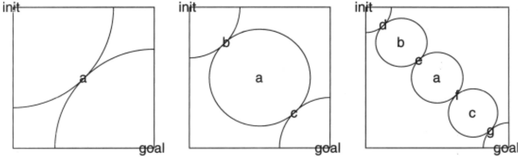
Figure 1 shows an idealized view of DCBDS. The left panel shows the final search horizons of the first bidi rectional search. Their intersection, node a, is the first node found on the optimal solution. The center panel shows the next two searches, from node a toward both the initial and goal states, adding the intersections at nodes b and c, respectively, to the solution. Finally, the right panel shows the next level of searches, adding nodes d, e, f, and g to the solution path. The reason the search frontiers look like circles and arcs of circles is that they represent an uniformed Dijkstra's algorithm, which doesn't know the direction to the goal.
3.1 Hirschberg's Algorithm
(Hirschberg, 1975] gives an algorithm for computing a maximal common subsequence of two character strings in linear space. It generates a two-dimensional matrix, with each of the original strings placed along one axis. An element of the matrix corresponds to a pair of initial substrings of the original stings, and contains the length of the maximal common subsequence of the substrings.
If n and m are the lengths of the original strings, the standard dynamic programming algorithm for this problem computes this matrix by scanning from left to right and top to bottom. This requires O(nm) time and O(nm) space. However, to compute any element of this matrix, we only need the value immediately to its left and immediately above it. Thus, we can compute the entire matrix by only storing two rows at a time, delet ing each row as soon as the next row is completed. In fact, only one row needs to be stored, since we can re place elements of the row as soon as they are used. Un fortunately, this only yields the length of the maximal common subsequence, and not the subsequence itself.
Hirschberg's algorithm computes the first half of the matrix from the top down, storing only one row at at time, and the second-half from the bottom up, again only storing one row. Then, given the two different ver sions of the middle row, one from each direction, he finds the column for which the sum of the two corresponding elements from each direction is a maximum. This point splits both original strings in two parts, and the algo rithm is then called recursively on the initial substrings, and on the final substrings.
The most important difference between DCBDS and Hirschberg's dynamic programming algorithm is that the latter scans the matrix in a predetermined systematic or der, while DCBDS expands nodes in order of cost. The dynamic programming algorithm can only be used when we can distinguish the ancestors of a node from its de scendents a priori. For example, it could be modified to find a lowest-cost path in a grid only if we restrict ourselves to minimum-length paths. DCBDS generalizes Hirschberg's dynamic programming algorithm to best first search of arbitrary graphs.
4 Complexity of DCBDS
In a problem of size O(nd), DCBDS reduces the space complexity from O(nd) to O(nd-l ), a very significant improvement. For example, if we can store ten mil lion nodes in memory, this increases the size of two dimensional problems we can solve from about 3, 000 x 3, 000 to about 2, 500, 000 x 2, 500,000 before memory is exhausted, since the maximum size of a search frontier is roughly the sum of the lengths of the axes. In practice, time is the limiting factor on large grids, and not space.
The asymptotic time complexity of Hirschberg's algo rithm, which only considers moves directly toward the goal, is the same as for the standard dynamic program ming algorithm, or O(nd) on ad-dimensional grid.
To analyze the time complexity of DCBDS, we model the search frontiers as circles and arcs of circles. A search frontier represents an Open list, and consists of a set of nodes whose costs from the start node are approximately equal, since the lowest-cost node is always expanded next. In our experiments, we only consider the moves up, down, left, and right. Thus, a set of nodes whose distance from the start are equal, in terms of number of edges, would be diamond shaped, with points at the four compass points. In this diamond, however, the nodes at the points only have a single path of minimal distance to them, but the nodes closest to the diagonals through the center have a great many different paths to them, all of minimal distance. Thus, the lowest-cost path to a node near the diagonal is likely to be much smaller than the lowest-cost path to a node near a point of the diamond. Since the frontier represents a set of nodes of nearly equal lowest-path cost, the frontier near the di agonals bows out relative to the points of the diamond, approximating the circular shape. In fact, our graphic simulation of best-first search on a grid shows that the search frontiers are roughly circular in shape.
The time complexity can be approximated by the number of nodes expanded, which is proportional to the area contained within the search frontier. Assume that · we have a square grid of size r x r, whose lowest-cost path is along the diagonal, which is of length r../2. The first bidirectional search, to determine point a in Figure 1, will cover two quarter circles, each of which is of ra dius r../2/2, for a total area of 2 · 1/ 47r(rv'2/2) 2 , which equals 1rr 2 /4. At the next level, we need two bidirec tional searches, one to determine point b, and one for point c. This generates two quarter circles from the ini tial and goal corners, plus the full circle centered at node a and reaching nodes b and c. This full circle will be gen erated twice, once to find node b, and once for node c. Thus, we generate 2 + 2 · 1/4 circles, each of which are of radius r../2/4, for a total area of 5/h(r../2/4)2 or 57rr 2 /16. At the third level, which generates nodes d, e, j, and g, we generate three full circles twice each, plus two quarter circles, all of radius r../2/8. In general, the set of searches at the nth level of recursion sweep out a total area of 2(2n-l- 1) + 2(1/4) circles, each of radius rv'2/2n, for a total area of
The total area of all the searches is the sum of these terms from n = 1 to the number of levels. As an upper bound, we can write it as the infinite sum
It is easy to show that this sum converges to one, so the total area, and hence time complexity of DCBDS, is 1rr 2 ·
To find a lowest-cost corner-to-corner path, the search frontier of Dijkstra's algorithm will spread in a circular arc from the initial corner to the goal corner, at which point the entire grid will usually be covered. Since the area of the grid is r 2 , the overhead of DCBDS compared to Dijkstra's algorithm is a constant factor of 1r.
We can perform the same analysis in three dimensions, the differences being that the searches sweep out volumes of spheres instead of areas of circles, the main diagonal of a cube is rv'3 instead of r../2, and the searches from the initial and goal states only generate eighths of a sphere, instead of quarters of a circle. In three dimensions, DCBDS generates a constant factor of 7rv'3/3 :::::J 1.8138 more nodes than Dijkstra's algorithm.
5 Experiments
We tested DCBDS on the problem of finding a lowest cost corner-to-corner path on a two-dimensional grid. Each edge of the grid is assigned a random cost, and the cost of a path is the sum of the edge costs along it. We considered the general lowest-cost problem, which allows moves away from the goal as well as toward the goal. Using a technique that allows us to efficiently jump around in a pseudo-random number sequence without generating all the intermediate values [Korf and Chick ering, 1996], we can search much larger random grids than we can store in memory.
| Size | Shortest Path | Solution Length | Total Nodes | Dijkstra Nodes | DCBDS Nodes | Ratio |
|---|---|---|---|---|---|---|
| 1,000 | 1,998 | 2,077 | 1,000,000 | 999,995 | 3,051,861 | 3.052 |
| 2,000 | 3,998 | 4,175 | 4,000,000 | 3,999,998 | 12,335,057 | 3.084 |
| 3,000 | 5,998 | 6,251 | 9,000,000 | 8,999,999 | 28,048,471 | 3.116 |
| 4,000 | 7,998 | 8,362 | 16,000,000 | 50,034,676 | 3.127 | |
| 5,000 | 9,998 | 10,493 | 25,000,000 | 78,430,448 | 3.137 | |
| 10,000 | 19,998 | 20,941 | 100,000,000 | 316,354,315 | 3.164 | |
| 20,000 | 39,998 | 41,852 | 400,000,000 | 1,274,142,047 | 3.185 | |
| 30,000 | 59,998 | 62,787 | 900,000,000 | 2,877,505,308 | 3.197 | |
| 40,000 | 79,998 | 83,595 | 1,600,000,000 | 5,118,240,659 | 3.199 | |
| 50,000 | 99,998 | 104,573 | 2,500,000,000 | 8,001,200,854 | 3.200 |
Table 1 shows our experimental results. For each grid size, we tested DCBDS on three different random prob lem instances, generated from different initial random seeds, and averaged the results for the problem instances. The results from one instance to the next are very simi lar, allowing such a small sample size. The first column gives the length of the grid in each dimension, and the second gives the number of edges in a shortest corner-to corner path, which is twice the grid size minus two. The third column gives the average number of edges in the lowest-cost corner-to-corner path. The reason some of these values are odd is because they are averages of three trials each. This data shows that in general a lowest-cost path is usually not a path of minimum length.
The fourth column gives the total number of nodes in the grid, which is the square of the grid size. The fifth column shows the average number of nodes expanded by Dijkstra's algorithm, for problems small enough to fit in memory. This data shows that Dijkstra's algorithm generates almost all the nodes in the grid. Since grids of size 4000 and greater are too large to fit in 128 megabytes of memory, we were unable to run Dijkstra's algorithm on these problems, and hence those entries are empty.
The sixth column shows the average number of nodes expanded by DCBDS, and the sixth column shows the ratio of the number of nodes expanded by DCBDS, di vided by the number of nodes that would be expanded by Dijkstra's algorithm, given sufficient memory. Even though we can't run Dijkstra's algorithm on problems greater than 3000 nodes on a side, we compute the ratio on the assumption that Dijkstra's algorithm would gen erate the ent ire grid, if there were sufficient memory. As predicted by our analysis, the number of nodes expanded by DCBDS is approximately 1r times the total number of grid points. This factor seems to increase slightly with increasing problem size, however.
The actual asymptotic running time of both algo rithms is 0 ( n 2 log n), where n is the size of the grid in one dimension. The n 2 term comes from the total number of nodes in the grid that must be examined. The log n term comes from the fact that both algorithms store the Open list as a heap, and the size of the Open list is 0( n), resulting in O(logn) time per node to access the heap.
Even though DCBDS expands over three times as many nodes as Dijkstra's algorithm, it takes less than twice as long to run. The main reason is that by sav ing the operators that have already been applied to a node, and not reapplying them, expanding a node takes less time than applying all operators and checking for duplicates in the Closed list. The grids of size 10,000 take DCBDS about two hours to run, and those of size 50,000 take about 3 days. The grids of size 50,000 require the storage of about 200,000 nodes, and with only 128 megabytes of memory, we can store over twelve million nodes. Thus, memory is no longer a constraint.
6 Further Work
An obvious source of waste in DCBDS is that most of the individual searches are performed twice. For example, in the center panel of Figure 1, the full circle centered at node a is searched twice, once to locate node b, and then again to locate node c. By performing the search for nodes b and c simultaneously, we would only have to generate the circle once. The same optimization can be applied to all the full-circle searches. Since most of the searches are full circles, this would reduce the time complexity by up to a factor of two, making DCBDS run almost as fast as Dijkstra's algorithm.
The drawback of this optimization is that it compli cates the algorithm. In particular, all the searches at the same level of recursion must be performed simulta neously. For example, in the right panel of Figure 1, the searches corresponding to the full circles must be inter leaved. This destroys the simple recursive structure of the algorithm, replacing it with an iterative outer loop with increasing numbers of interleaved searches in each iteration. In addition, some of these searches will termi nate before others, and some may not even be necessary.
Our current implementation continues executing re cursive bidirectional searches until the initial and goal nodes are the same. Another obvious optimization would be to terminate the recursion when the problem size is small enough that there is sufficient memory to hold the entire subgrid in memory, and then execute Dijkstra's al gorithm at that point. Since our analysis suggests that the lower-level searches in the recursion hierarchy con tribute diminishingly less to the overall time, this opti mization may not result in significant savings.
The idea of storing only the Open list in memory sug gests yet another algorithm for this problem. What we could do is to execute a single pass of Dijkstra's algo rithm, saving only the Open list, but writing out each node as it is expanded or closed to a secondary storage device, such as disk or magnetic tape, along with its par ent node on an optimal path from the root. Then, once the search is completed, we r.econstruct the solution path by scanning the file of closed nodes backwards, looking for the parent of the goal node, then the parent of that node, etc. Since nodes are expanded in nondecreasing order of their cost, we are guaranteed that the complete solution path can be reconstructed in a single backward pass through the file of closed nodes.
The advantage of this approach is that the capacity of most secondary storage devices is considerably greater than that of main memory, and we can access the device sequentially rather than randomly. Unfortunately, most such devices can't be read backwards very efficiently. The best we could do would be to simulate this by read ing a disk or tape file in blocks large enough to fit in main memory, and then access these blocks in reverse or der. Given the efficiency of DCBDS, and the slow speed of secondary storage devices, however, it's unlikely that this will lead to a faster algorithm.
7 Conclusions
We generalized Hirschberg's dynamic programming al gorithm to reduce the memory requirement of best-first search in arbitrary graphs with cycles. The most impor tant difference between DCBDS and the dynamic pro gramming algorithm is that the latter only works when we know a priori which neighbors of a node can be its ancestors and descendents, respectively, while DCBDS requires no such knowledge. For example, Hirschberg's algorithm can find a lowest-cost path in a grid if we only allow edges in the direction of the goal, whereas DCBDS allows arbitrary solution paths. Our experiments show that in general the lowest-cost path in a two-dimensional grid is not of minimal length.
DCBDS is most effective on polynomial-sized prob lems that are too big to fit in memory. In such prob lems, it reduces the memory requirement from O(nd) to O(nd-l ). Our analysis suggests that the time cost of this reduction is only a constant factor of 1r in two dimen sions, which is supported by our experimental results. In three dimensions, our analysis predicts a constant over head of 7rv'3/3 ~ 1.8138. Further optimizations could reduce these constants by up to a factor of two, and ad ditional constant savings may reduce the actual running time to no more that traditional best-first search.
While we used Dijkstra's algorithm in our experi ments, the generalization of DCBDS to A* is straightfor ward. A* may prune more of the search space, allowing larger problems to be solved, but it is also space-bound in practice, and hence will benefit from this technique.
The traditional drawback of bidirectional search has been its memory requirements. Ironically, DCBDS shows that bidirectional search can be used to save mem ory, and has the potential to revive study of this area.
8 Acknowledgements
Thanks to Toru Ishida and Teruhisa Miura for introduc ing me to the gene sequence alignment problem. Thanks to Hania Gajewska for developing the graphics code. This research was supported by NSF grant IRI-9619447.
@inproceedings{ijcai1999p168,
  title     = {A Divide and Conquer Bidirectional Search: First Results},
  author    = {Korf, Richard E.},
  booktitle = {Proceedings of the Sixteenth International Joint Conference on
               Artificial Intelligence, {IJCAI-99}},
  publisher = {International Joint Conferences on Artificial Intelligence},
  editor    = {Thomas Dean},
  pages     = {1184--1190},
  year      = {1999},
  note      = {Search},
  url       = {https://ijcai.org/proceedings/1999/168},
}
TY - CPAPER TI - A Divide and Conquer Bidirectional Search: First Results AU - Korf, Richard E. T2 - Proceedings of the Sixteenth International Joint Conference on Artificial Intelligence, IJCAI-99 PB - International Joint Conferences on Artificial Intelligence PY - 1999 SP - 1184 EP - 1190 UR - https://ijcai.org/proceedings/1999/168 ER -Copied
Machine-readable versions of this paper, for tools and AI agents:





