
Computational Complexity of Planning and Approximate Planning in Presence of Incompleteness
Proceedings of the Sixteenth International Joint Conference on Artificial Intelligence. Planning and Scheduling. Pages 948-954.
© 1999 International Joint Conferences on Artificial Intelligence
Abstract
In t he last several yea rs th e co mputational complexity of classical planning and HTN planning have b ee n s tudi ed . But in both cases it is assumed that the planner has complete knowledge about th e initial state. Recently, th ere has b ee n proposal to use 'sensing ' actions to plan in presence of incompleteness . In this paper we study the complexity of planning in such cases. In our study we use the action description language A proposed in 1993 by M. Gelfond and V. Lifschitz and its extensions. The language A allows planning in the situations with complete information. It is known t h at, if we consider only plans of feasible (polynomial) length , the planning problem for such situations is NP-complete : even checking whether a given objective is attainable from a g iv en initi al state is NP- complete. In this paper, we show that th e planning problem in presen ce of incompleteness is indeed hard er : it belongs to the next level of complexity hierarchy (in precise terms, it is I:2P-complete) . To overcome th e complexity of this problem, C. Baral and T . Son have proposed several approximations. We show that under certain conditions, one of th ese approximations - 0-approximation - mak es the problem NP- complete (thus indeed redu cing its complexity).
- [Baral and Son , 1997] C. Baral and T. Son, "Approxi- mate reasoning about actions in presence of sensing and incomplete information", In: Proc. of Inter- national Logic Programming Symposium (ILPS 1 97}, 1997, pp. 387-401.
- [Erol et al., 1995] K. Erol, D. S. Nau, and V. S. Subrah- manian, "Complexity, decidability and undecidabil- ity results for domain-independent planning", Arti- ficial Intelligence, 1995 , Vol. 76 , pp. 75-88 (detailed proofs are given in the University of Maryland Tech- nical Report CS-TR-2797 (also listed as UMIACS- TR-91-154 and SRC-91-96).
- [Gelfond and Lifschitz, 1993] M. Gelfond and V. Lifs- chitz, "Representing actions and change by logic programs", J. of Logic Programming , 1993, Vol. 17, pp. 301-322.
- [Liberatore, 1997] P. Liberatore, "The complexity of the language A", Electronic Transactions on Ar- tificial Intelligence, 1997, Vol. 1, pp. 13-28 (http:/ /www.ep.liu.se/ejjetai/1997 /02). Link
- [Littman, 1997] M. Littman, "Probabilistic proposi- tional planning: representation and complexity", AAAI'97, pp. 748-754.
- [Moore, 1985] R. Moore, ''A formal theory of knowledge and action." In J. Hobbs and R. Moore, editors, Formal theories of the commonsense world. Ablex, Norwood, NJ, 1985.
- [Papadimitriou, 1994] C. H. Papadimitriou, Computa- tional Complexity , Addison-Wesley, Reading , MA , 1994.
- [S cher! and Levesque, 1993] R . Scher! and H. Levesque, "The frame problem and knowledge producing ac- tions. " In KR 93, pages 689-695, 1993.
- [Son and Baral, 1998] T. Son, and C. Baral, Formaliz- ing sensing actions -a transition function based approach, University of Texas at El Paso , Depart- ment of Computer Science, Technical Report, 1998 (http:// cs. utep.edu / chitta/ chitta. html) . Link
- BARAL. KREINOVICH, AND TREJO
References were extracted automatically from the PDF and may contain errors.
Full text extracted automatically from the PDF; figures, tables and equations may differ. The PDF is the version of record.
1 Introduction
The action description language A proposed in 1993 by M. Gelfond and V. Lifschitz [Gelfond and Lifschitz, 1993] and its successors have made it easier to understand the fundamentals (such as inertia, ramification, qualifica tion, concurrency, sensing, etc.) involved in formalizing actions and their effects on a world, without getting into the details of particular logics. In this paper , we will be analyzing the complexity of planning based on this language and its extensions; let us , therefore, start with a brief description of this language.
1.1 Language A: brief reminder
In the language A , we start with a finite list of proper ties (fluents) 11 , ... , fn which describe possible proper ties of a state. A state is then defined as a finite set of fluents, e.g., {} or {11, /3}. We are assuming that we have a complete knowledge about the initial state: e.g., {11 , /3} means that in the initial state, properties 11 and h are true, while all the other properties h, /4 , .. . are false . The properties of the initial state are described by formulas of the type
where F is a fluent literal, i.e., either a fluent /; or its negation --.,j; .
To describe possible changes of states, we need a finite set of actions. In the language A, the effect of each action a can be described by formulas of the type
where F, Ft , .. . , Fm are fluent literals. A reason ably straightforward semantics describes how the state changes after an action:
- if before the action a, the literals F1 , ... , Fm were true, and the domain description contains a rule ac cording to which a causes F if F1, ... , Fm, then this rule is activated, and after the action a , F becomes true; thus , for some fluents /;, we will conclude /; and for some other, that 'fi holds in the next state;
- if for some fluent /;, no activated rule enables us to conclude that / ; is true or false , this means that the action a does not change the truth of this fluent ; therefore, /; is true in a new state if and only if it is true in the old state.
Formally, a domain description D is a finite set of value propositions of the type initially F (which describe the initial state) , and a finite set of effect propositions of the type "a causes F if F1, ... , Fm" (which describe results of actions) . A state s is a finite set of fluents. The initial state s0 consists of all the fluents J; for which the corresponding value proposition initially / ; is contained in the domain description. We say that a fluent / ; holds in s if J; E s; otherwise, we say that --,j; holds in s. The transition function Resv (a, s) which describes the effect of an action a on a state s is defined as follows :
- we say that an effect proposition "a causes F if F1 , ... , Fm" is activated in a state s if all m fluent literals F1 , ... , Fm hold in s;
- we define VJ(a, s) as the set of all fluents fi for which a rule "a causes fi if F1 , ... , Fm" is activated m s;
- similarly, we define v; (a, s) as the set of all fluents fi for which a rule "a causes ·fi if F1, .. . , Fm" is activated in s;
- if VJ(a, s) n v;(a, s) :f.~, we say that the result of the action a is undefined;
- if the result of the action a is not undefined in a states (i.e., if V.J"(a,s) n VD"(a,s) = 0), we define ResD(a, s) = (s U V.J"(a, s)) \ VD"(a, s).
A plan pis defined as a sequence of actions [a1, ... , am]. The result ResD(P, s) of applying a plan p to the initial state so is defined as
The planning problem is: given a domain D and a de sired fluent literal F, to find a plan which leads to the state in which F is true. (More complicated goals can be reformulated in these terms.)
1.2 An extension of language A which describes sensing actions: brief reminder
The language A describes planning in the situations with complete information, when we know exactly which flu ents hold in the initial state and which don't. In real life, we often have only partial information about the initial state: about some fluents, we know that they are true in the initial state, about some other fluents, we know that they are false in the initial state; and it is also pos sible that about some fluents, we do not know whether they are initially true or false. In such situations, the required action depends on the state: e.g., if we want the door closed, the required action depends on whether the door was initially open (then we close it), or it was already closed (then we do nothing). Therefore, for these situations, we must include sensing actions- e.g., an ac tion checki which checks whether the fluent fi holds in a given state - to our list of actions, and allow conditional plans, i.e., plans in which the next action depends on the result of the previous sensing action.
Some fluents may be difficult to detect, so we may have sensing actions only for some fluents; some real life sensing actions may sense several fluents at a time. In view of these possibilities, the precise formulation of this language is as follows 1 . In the domain description D, in addition to value propositions and effect proposi tions, we can also have sensing propositions, of the type "a determines N'. A k-state is defined as pair (s, ~), where s is the actual state, and~ is the set of all possible states which are consistent with our current knowledge. Initially, the set ~0 consists of all the states s for which:
1 The formulation given here is based on earlier work of formalizing sensing actions in [Moore, 1985; Scher! and Levesque, 1993].
- a fluent fi is true (fi E s) if the domain description D contains the proposition "i nitially N';
- a fluent fi is false (fi tf. s) if the domain description D contains the proposition "initially ·N' .
If neither the proposition "initially N', nor the proposi tion "initially ·Ji'' are in the domain description, then 2; 0 contains states with fi true and with fi false. The actual initial state s0 can be any state from the set I;o. The transition function is defined as follows:
- for proper (non-sensing) actions, (s, I;) is mapped into
(ResD(a, s), ResD(a, I;)), where:
- ResD(a, s) is defined as in the case of complete information, and
- ResD(a, I;)= {ResD(a, s') Is' E I;}.
- for a sensing action a which senses fluents fl, ... , fk - i.e., for which sensing propositions "a determines fi" belong to the domain D - the actual state s remains unchanged while I; is down to only those states which have the same values of fi ass: (s, I;)-+ (s, I;'), where
In the presence of sensing, an action plan is no longer a pre-determined sequence of actions: if one of these actions is sensing, then the next action may depend on the result of that sensing. In general, the choice of a next action may depend on the results of all previous sensing actions. Such an action plan is called conditional.
Examples have shown that adding sensing actions in creases the computational complexity of the problem. In this paper, we show that the .corresponding planning problem is indeed harder: it belongs to the next level of complexity hierarchy (in precise terms, it is I;2P complete).
1.3 The notion of a 0-approximation
To overcome the complexity of this problem, C. Baral and T. Son have proposed several approximations , whose plans are always correct but which can miss a plan. The first approximation- called a-approximation - is as fol lows: An a-state (approximate state) s is a finite set of fluent literals (i.e., fluents and their negations). The initial a-state so consists of all the fluent literals F for which the corresponding value proposition "initially F" is contained in the domain description. We say that:
- a fluent fi if true in s is fi E s;
- a fluent fi if false in s is ·fi E s;
- a fluent fi if unknown in s is neither fi E s, not ·fi E s.
The transition function ResD(a, s) which describes the effect of a proper action a on an a-state s is defined as follows:
- we say that an effect proposition "a causes F if F1, ... , F m " is activated in an a-state s if all m fluent literals F1, ... , Fm hold in s;
- we say that an effect proposition "a causes F if F1 , ... , F m" is possibly activated in an a-state s if all m fluent literals F1 , . . . , Fm possibly hold in s (i.e., are either true, or unknown in s);
- ~e define VD(a, s) as the set of all fluent literals F for which a rule "a causes F if F1 , ... , Fm" is acti vated in s, and no rule "--,a causes F if F1 , ... , Fm" is possibly activated in s;
- we then define ResD(a , s) as
For sensing actions, the result of applying a to an a-state s simply means adding, to the a-state, the fluent literals which turned out to be true as a result of this sensing action.
2 Results
2.1 What kind of planning problems we are interested in
Informally speaking, we are interested in the following problem:
- given a domain description (i.e ., the description of the initial state and of possible consequences of dif ferent actions) and a goal (i.e. , a fluent which we want to be true) ,
- determine whether it is possible to achieve this goal (i.e., whether there exists a plan which achieves this goal).
We are interested in analyzing the computational com plexity of the planning problem, i.e., analyzing the com putation time which is necessary to solve this problem.
Ideally, we want to find cases in which the planning problem can be solved by a feasible algorithm, i.e., by an algorithm U whose computational time tu ( w) on each in put w is bounded by a polynomial p(lwl) of the length lwl of the input w: tu(x) ~ p(lwl) (this length can be measured bit-wise or symbol-wise. Problems ·which can be solved by such polynomial-time algorithms are called problems from the class P (where P stands for polynomial-time). If we cannot find a polynomial-time algorithm, then at least we would like to have an algo rithm which is as close to the class of feasible algorithms as possible.
In short , we are interested in restricting the time which it takes to check whether the planning problem is solv able. This interest is justified because in planning appli cations we often want the resulting plan to be produced in real time, and if it is not possible to produce such a plan, we would like to know about this impossibility as early as possible, so that we will be able to add new actions (or simply give up). Since we are operating in a time-bounded environment, we should worry not only about the time for computing the plan, but we should also worry about the time that it takes to actually im plement the plan . If an action plan consists of a sequence of 2 2 " actions, then this plan is not feasible. It is there fore reasonable to restrict ourselves to f easible plans, i.e., by plans u whose length lui (= number of actions in it) is bounded by a polynomial p(lwl) of the input w. With this feasibility in mind, we can now formulate the above planning problem in precise terms :
- given: a polynomial p(n) 2: n, a domain descrip tion D (i .e., the description of the initial state and of possible consequences of different actions) and a goal f (i .e., a fluent which we want to be true) ,
- determine whether it is possible to feasibly achieve this goal, i.e., whether there exists a feasible plan u (with lui~ p(IDI)) which achieves this goal.
We are interested in analyzing the computational com plexity of this planning problem.
2.2 Complexity of the planning problem for situations with complete information
For situations with complete information, the above planning problem is NP-complete:
Theorem 1. For situations with complete information, the planning problem is NP-complete.
Comments.
- This result is similar to the result of Liberatore [Lib eratore, 1997) . The main difference is that Libera tore considers arbitrary queries from the language A , while we only consider queries about the exis tence of a feasible action plan.
- The result of Liberatore is preceded by the results of Erol et al [Erol et al., 1995) where they study com plexity of STRIPS. Here we use A and its extensions instead of STRIPS as to the best of our knowledge there has not been any formal treatment of exten sions of STRIPS dealing with sensing actions.
- For lack of space we are not able to present all the proofs in this paper .
- The problem remains NP-complete even if we con sider the planning problems with a fixed finite num ber of actions: even with two actions. If we only allow a single action, then there is no planning any more: the only possible plan is, in any state, to ap ply this only possible action and check whether we have achieved our goal yet; the corresponding "plan ning" problem is, of course, solvable in polynomial time.
2.3 Useful complexity notions
For situations with incomplete information, the planning problem is more complicated - actually, belongs to the next levels of polynomial hierarchy; see the exact results below. For precise definitions of the polynomial hierar chy, see, e.g., [Papadimitriou, 1994) . Crudely speaking, a decision problem is a problem of deciding whether a given input w satisfies a certain property P (i.e., in set theoretic terms, whether it belongs to the corresponding set 5= {wiP(w)}).
- A decision problem belongs to the class P if there is a feasible (polynomial-time) algorithm for solving this problem.
- A problem belongs to the class NP if the checked formula w E S (equivalently, P(w)) can be rep resented as 3uP(u, w), where P(u, w) is a feasible property, and the quantifier runs over words of fea sible length (i.e., of length limited by some given polynomial of the length of the input). The class NP is also denoted by ~1 P to indicate that formu las from this class can be defined by adding 1 exis tential quantifier (hence ~ and 1) to a polynomial predicate (P).
- A problem belongs to the class coNP if the checked formula w E S (equivalently, P(w)) can be rep resented as VuP(u, w), where P(u, w) is a feasible property, and the quantifier runs over words of fea sible length (i.e., of length limited by some given polynomial of the length of the input). The class coNP is also denoted by II1P to indicate that for mulas from this class can be defined by adding 1 universal quantifier (hence II and 1) to a polyno mial predicate (hence P).
- For every positive integer k, a problem be longs to the class ~kp if the checked for mula w E S (equivalently, P( w)) can be rep resented as 3u1Vu2 ... P(ut,u2,· ··,uk.w), where P(u1, . .. , uk, w) is a feasible property, and all k quantifiers run over words of feasible length (i.e., of length limited by some given polynomial of the length of the input).
- Similarly, for every positive integer k, a prob lem belongs to the class IIkP if the checked for mula w E S (equivalently, P( w)) can be rep resented as 'iut3Uz .. . P(ut,u2, ... ,uk.w), where P( Ut, ... , uk, w) is a feasible property, and all k quantifiers run over words of feasible length (i.e., of length limited by some given polynomial of the length of the input).
- All these classes ~k P and Ilk P are subclasses of a larger class PSPACE formed by problems which can be solved by a polynomial-space algorithm. It is known (see, e.g., [Papadimitriou, 1994]) that this class can be equivalently reformulated as a class of problems for which the checked formula w E S (equivalently, P( w)) can be represented as Vul:Ju2 ... P(ut, u2, . . . , Uk , w), where the number of quantifiers k is bounded by a polynomial of the length of the input, P( u1, . . . , Uk, w) is a feasible property, and all k quantifiers run over words of feasible length (i.e., of length limited by some given polynomialof the length of the input).
A problem is called complete in a certain class if crudely speaking, this is the toughest problem in this class (so that any other general problem from this class can be reduced to it by a feasible-time reduction). It is still not known (1998) whether we can solve any prob lem from the class NP in polynomial time (i.e., in precise terms, whether NP=P) . However, it is widely believed that we cannot, i.e., that NP:f:P. It is also believed that to solve a NP-complete or a coNP-complete problem, we need exponential time ~ 2n, and that solving a com plete problem from one of the second-level classes ~2 P or II2P requires more computation time than solving NP complete problems (and solving complete problems from the class PSPACE takes even longer).
2.4 Complexity of the planning problem for situations with incomplete information: situations with no sensing actions
Let us start our analysis with the case of no sensing.
Theorem 2. For situations with incomplete informa tion and without sensing, the planning problem is ~2P complete.
Proof. The problem is to check the existence of a feasible-length action plan u1 for which, for every set of values u2 of the unknown fiuents, Ut is successful, i.e., we check whether :lu1Vu2P(ut,u2,w). Once we know u1 and u2 (i .e., once we know the initial state and the actions), we can determine, step-by-step, all follow ing states, and thus check, in polynomial time, whether in the final state, the desired predicate is true. So, P E ~2P.
To show that P is complete, we reduce, to P , a known complete propositional problem of checking :lx1 .. . 3xm'iXm+l ... 'ixn F, (xi are propositional vari ables, F is a propositional formula). To reduce it to P, we first parse F, i.e., we represent computing F as a sequence of elementary steps, on each of which we apply &, V, or -, to compute the intermediate results Xn+l, ... ,xN: e.g., to compute (x1 Vx2)&(x1 V·x2), we compute X3 := Xt V x2, etc. In our planning problem, we take two actions a and a-, and fiuents x1, ... , xN , s0 , s1, ... , SN (meaning: Si is true iff time= i). Initially, s0 is true, all other Si are false; x N is false, all other Xi are unknown; goal: XN ="true". In the first m moments of time, we select variables x 1, . .. , Xm: a selects Xi , a selects ·xi: "a causes Xi if Si-t" (same for a-); also, ev ery action increases time by one: e.g. , a causes Si if Si-1 and causes ·Si-1 if Si-l · In moments k = n + 1, ... , N, we "compute" xk: e.g., ifxk := Xf&x,, then a causes Xk if Sk-1, Xf, x,, causes · Xk if sk-1, ·Xj, and causes ·Xk if Sk-1, ·Xs ( + rules which increase time by 1) . A plan exists iff there exist values x1, ... , Xm for which, for all Xm+l, ... , Xn, F is true. The reduction proves that P is complete.
The problem remains ~2 P-complete even if we consider the planning problems with a fixed finite number of ac tions: even with two actions.
Theorem 3. For situations with incomplete informa tion and without sensing, the a-approximation to the planning problem is NP- complete.
In other words, the use of a-approximation cuts off one level from the complexity. So, for this problem, a approximation is indeed computationally very efficient .
This reduct ion is in good accordance with our intuitive understanding of this problem and its a-approximation:
- In the case of complete information, to represent a state, we must know which fluents are true and which are false. Therefore , a state can be uniquely described by a subset of the set of all the fluents - namely, the subset consisting of those fiuents which are true in this state. The total number of states is therefore equal to the total number of such subsets , i.e., to 2F (where F is the total number of fiuents).
- In the case of incomplete information, we, in gen eral, do not know which states the system is. So, a state of our knowledge (called a k-stat e in [Son and Baral , 1998]) can be represented by a set of possible complete-information states. Therefore, the num ber of all possible k-states is equal to the number of all possible subsets of the set of all complete information states, i.e., to 2 2 F.
- In a-approximation, an a-state is represented by stating which fiuents are true, which are false, and which are unknown. For each of F fluents , there are three different possibilities, so totally, in this approximation, we have 3F possible a-states.
So, going from a full problem to its a-approximation decreases the number of possible "states" from doubly exponential 2 2 F to singly exponential 3F . Since plan ning involves analyzing different possible states, it is no wonder that for a-approximation, the computation time should also be smaller. Again, this argument is not a proof of Theorem 3, but this argument makes the result of Theorem 3 intuitively reasonable.
2.5 Complexity of the planning problem for situations with incomplete information: situations with sensing
Let us now consider what will happen if we allow sens ing actions. If we allow unlimited sensing, then the situ at ion changes radically: the planning problem becomes so much more complicated that a-approximation is not helping anymore:
Theorem 4. For situations with incomplete in formation and with sensing, the planning problem is PSPACE-complete.
Theorem 5. For situations with incomplete informa tion and with sensing, the a-approximation to the plan ning problem is PSPACE-complet e.
The proofs are similar to [Littman , 1997] . Both the planning problem itself and its a-approximation remain PSPACE-complete even if we consider the planning problems with a fixed finite number of actions: even with two proper actions and a single sensing action which re veals the truth value of only one fluent - but we are al lowed to repeat this sensing action at different moments of time.
In many real life control and planning situations, it is desirable to monitor the environment continuously, and to make sensing actions all the time. However, this ne cessity is caused by the fact that in many real-life sit uations, the consequences of each action are only sta tistically known, so we need to constantly monitor the situation to find out the actual state. In this paper, we consider the situations in which the result of each action is uniquely determined by this action and by the initial state. In such idealized situations, there is no such need for a constant monitoring. It therefore makes sense to allow only a limited repetition of sensing actions in an action plan. With such a limitation, the complexity of planning drops back, and a-approximation starts helping agam:
Definition 1. Let k be a positive integer.
- We say that a sensing action is k-limited if it reveals the values of no more than k fluents.
- We say that an action plan is k-bounded if it has no more than k sensing actions.
Theorem 6. For any given k , for situations with incom plete information and with k-limited sensing actions, the problem of checking the existence of a k-bounded action plan is ~2 P-complete.
Theorem 7. For any given k, for situations with in complete information and with k-limited sensing actions, the problem of checking the existence of a k-bounded a approximation action plan is NP-complete.
Comments.
- The same result holds if instead of assuming that k is a constant, we allow k to grow as Jlog(IDI) (i .e., as a square root of the logarithm of the length of the input).
- A difficulty with the general situation with incom plete information comes from the fact that we do not know the exact states, i.e., we do not know the values of all the fiuents. It is therefore reason able to analyze the situations with full sensing, i.e., situations in which , for every fluent f ;, we have a sensing action check; which reveals the value of this fluent . Full sensing does make the planning prob lem simpler, although not that simpler so that a approximation will help :
Theorem 8. For situations with incomplete informa tion and with full sensing, the planning problem is IT2P complete.
Theorem 9. For situations with incomplete informa tion and with full sensing, the a-approximation to the planning problem is IT2P-complete .
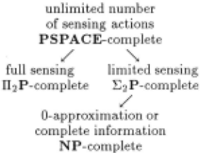
These results can be represented by the following table:
| II exact planning | 0-approximation | |
|---|---|---|
| complete information | NP-complete | NP-complete |
| partial informat-, ion, no sensing | :E2P-complete | NP-complete |
| limited number of sensing actions | :E2P-complete | NP-complete |
| unlimited number of sensing actions | PSPACE- complete | PSPACE- complete |
| partial informat- ion, full sensing | II 2 P -complete | II2P-complete |
2.6 Auxiliary result: !-approximation is coNP-complete
In addition to 0-approximation, the authors of [Baral and Son, 1997; Son and Baral, 1998] considered other types of approximations, including the so-called } approximation. In !-approximation, partial states are defined in the same manner as for 0-approximation: i.e., as lists of fluents and their negations. However, the re sult of a (proper) action a on an a-state s is defined differently: in this new approximation, a fluent literal F (fluent or its negation) is true after applying a to s if and only if F is true in all possible complete states comple menting s. Then, as a new a-state Resv(a, s), we take the set of all fluent literals which are true after applying a.
In this section, we will show that this new definition increases the computational complexity of an approxi mation. Namely, while for 0-approximation, computing the next a-state Resv(a, s) was a polynomial-time pro cedure, for !-approximation, computing the next state is already a coNP-complete problem:
Theorem 10. (!-approximation) The problem of check ing, for a given a-state s 1 for a given action a 1 and for a given fluent / 1 whether f is true in Resv(a, s), is coNP complete.
Comments.
- An w-approximation is defined in a similar man ner, except that in an w-approximation, the result Resv(a, s) is defined not after a single action a, but after a sequence of proper actions between two sens ing actions. In the particular case when there is ex actly one proper action between the two sensing ac tions, w-approximation reduces to !-approximation. Therefore, w-approximation is also at least as com plicated as coNP-complete problems.
- These results show that if we want an approx imation to decrease the computational complex ity of the planning problem, then (at least from the viewpoint of the worst-case complexity) a approximation is preferable to !-approximation and w-approximation.
@inproceedings{ijcai1999p135,
  title     = {Computational Complexity of Planning and Approximate Planning in Presence of Incompleteness},
  author    = {Baral, Chitta and Kreinovich, Vladik and Trejo, Raul},
  booktitle = {Proceedings of the Sixteenth International Joint Conference on
               Artificial Intelligence, {IJCAI-99}},
  publisher = {International Joint Conferences on Artificial Intelligence},
  editor    = {Thomas Dean},
  pages     = {948--954},
  year      = {1999},
  note      = {Planning and Scheduling},
  url       = {https://ijcai.org/proceedings/1999/135},
}
TY - CPAPER TI - Computational Complexity of Planning and Approximate Planning in Presence of Incompleteness AU - Baral, Chitta AU - Kreinovich, Vladik AU - Trejo, Raul T2 - Proceedings of the Sixteenth International Joint Conference on Artificial Intelligence, IJCAI-99 PB - International Joint Conferences on Artificial Intelligence PY - 1999 SP - 948 EP - 954 UR - https://ijcai.org/proceedings/1999/135 ER -Copied
Machine-readable versions of this paper, for tools and AI agents:





