Convergence of Reinforcement Learning with General Function Approximators

1 Introduction

Reinforcement learning (RL) is a widely used method for learning to make decisions in complex, uncertain environ­ ments. Typically, an RL agent perceives and acts in an en­ vironment, receiving rewards that provide some indication of the quality of its actions. The agent's goal is to maximize the sum of rewards received. RL algorithms work by learn­ ing a value function that describes the long-term expected sum of rewards from each state; alternatively, they can learn a Q-function describing the value of each actio~ .in each state. These functions can then be used to make decisiOns.

Temporal-difference (TD) learning [Sutton, 1988] is a com­ monly used family of reinforcement learning methods. TD al­ gorithms operate by adjusting the value function to be locally consistent. When used with function approximators, such as neural networks, that provide a compact parameterized repre­ sentation of the value function, TD methods can solve real­ world problems with very large state spaces. Because of this, one would like to know if such algorithms can be guaranteed to work-i.e., to converge and to return optimal solutions.

The theoretical study of RL algorithms usually divides the problem into two aspects: exploration policies that can guar­ antee complete coverage of the environment, and value deter­ mination to find the value function that corresponds to a given policy. This paper concentrates on the second aspect. Prior work [Jaakkola et al., 1995] has established convergence of TD-learning with probability 1 when the value function is rep­ resented as a table where each state has its own entry. For large state spaces, however, compact parametric representa­ tions are required; for such representations, we are .interest~d in whether an algorithm will converge to the functiOn that IS closest, by some metric, to the true value function (a form of agnostic learning). Gordon [ 1995] proved that TD converges in this sense for representations called "averagers" on which the TD update is a max-norm contraction (see Section 2) .. Tsit­ siklis and van Roy [ 1996] proved convergence and established error bounds for TD(>.) with linear combinations of fixed ba­ sis functions.

With nonlinear representations, such as neural networks, TD has been observed to give suboptimal solutions [Bert­ sekas and Tsitsiklis, 1996] or even to diverge. This is a se­ rious problem since most real problems require nonlinearity. Baird [1995] introduced residual algorithms, for which con­ vergence can be proved when combined with a gradient de­ scent learning method (such as used with neural networks). Unfortunately the error in the resulting approximation can be arbitrarily large and furthermore the method requires two in­ dependent visits to each sampled state.

This paper describes the Bridge algorithm, a new RL method for which we establish convergence and error bounds with any agnostically learnable representation.

Section 2 provides the necessary definitions and notation. Section 3 explains the problem of nonconvergence and pro­ vides examples of this with TD. Section 4 outlines the Bridge algorithm, sketches the proof of convergence, and shows how it solves the examples for which TD fails. Section 5 briefly covers additional results on convergence to local optima for any representation and on the us~ of PAC~Iearning the?ry. Section 6 mentions some alternative techmques one rrught consider. The paper is necessarily technically dense given the space restrictions. The results, ho~ever, should. ~e of broad interest to the AI and machine learnmg commumt1es.

2 Definitions

2.1 MDP

A Markov decision process M = (S, A, p, r , 1) is a set of states S, a set of actions A, transition probability distributions p( ·lx, a) that define the next state distribution given a current state x and action a, reward distributions r( ·lx, a) that define the distribution of real-valued reward received upon execut­ ing a in x, and a discount factor 1 E (0, 1). Since we are in­ terested in the problem of value determination, we assume we are given a fixed policy (choice of action at each state). When executing only this fixed policy, the MDP actually becomes a Markov chain, and we may therefore also write the transition probabilities asp( ·lx) and the reward distributions as r( ·lx ). We assume that we are able to define the stationary distribu­ tion 1r of the resulting Markov chain and also that the rewards lie in the range [-Rmax, Rmax]·

Let (X 1 , X 2, X 3, ... ) be a random trace in the Markov chain startingfrom x, i.e. X1 = x,X2 hasdistributionp(-IX1) and Xk has distribution p(-IXk_I) . Let (R1, R2, R3, ... )be the observed random rewards, i.e. Rk has distribution r(-IXk) · Define the true value function v· at a state x to be the ex­ pected, discounted reward to go from state x:

The problem of value determination is to determine the true value function or a good approximation to it. Classical TD so­ lutions have made use of the backup operator T, which takes an approximation V and produces a better approximation

An operator A is said to be a contraction with factor ( < 1 under some norm II · II if

If ( = 1, A is said to be a nonexpansion. If we define the max-norm to be IIVIImax = maxxES V( x) and the 1r-norm to be IIVII .. = [Lx ES V( x) 2 1r(x)FI 2 , then Tis a contraction with factor 1 and fixed point V* under both max-norm and 1r-norm [Tsitsiklis and Van Roy, 1996]. Therefore repeated application ofT (i.e. the iterative process V n+l = TV n) converges to v ·. We will use Ti to represent the operator T applied j times.

If the transition probabilities p and reward distributions r are known, then it is possible to compute TV directly from its definition. However, if p and r are not known, then it is not possible to compute the expectation in the definition ofT. In this case, by observing a sequence of states and rewards in the Markov chain, we can form an unbiased estimate of TV. Specifically, if we observe state x and reward r followed by state x2 , then the observed backed-up value, r + 1V(x2), is an unbiased estimate ofTV(x ). Formally we define Pj. (·lx) to be the conditional probability density of observed backed­ up values from state x:

where R1 and X2 are, as defined above, random variables with distributions r(-l x) and p(-l x) respectively. Thus if a random variable Y has associated density Pj. (-l x) then E(Y] = TV(x). Similarly, we define Pj:i(-lx) to be the conditional probability density of j-step backed-up values ob­ served from state x.

2.2 Function Approximation

As state spaces becomes large or even infinite, it becomes in­ feasible to tabulate the value function for each state x, and we must resort to function approximation. Our approximation scheme consists of a hypothesis class 1l of representable func­ tions and a learning operator 111£ which maps arbitrary value functions to functions in 1l.

The standard T based approaches that use function approx­ imation essentially compute or approximately compute the iterative process Vn+l = 111-lTVn. In practice, the 111£T mapping usually cannot be performed exactly because, even if we have access to the necessary expectation to compute TV ( x) exactly, it is infeasible to do so for all states x. Thus we perform an approximate mapping using samples. We will take the state sample distribution to be the stationary distri­ bution 1r . In general when we cannot compute TV(x) ex­ actly, we approximate 111£TV by generating samples (x, y) with sample distribution

'

and passing them to a learning algorithm for 1l. The joint probability density Pj. (from which we generate the samples) simply combines 1r (from which we sample the state x) with the conditional probability density Pj. ( ·lx) (from which we generate an estimate y for TV(x)).

In this paper we focus on agnostic learning. In this case, the learning operator 111£ seeks the hypothesis h that best matches the target function V, even though typically the target func­ tion is not in the hypothesis class. If we measure distance us­ ing the 1r-norm, then we can define the learning operator for agnostic learning to be:

As already mentioned, in the typical case we do not have access to the exact function V to be learned, but rather we can draw samples ( x , y) from a sample distribution P such that the expected value of the conditional distribution P( ·lx) is V(x). If, in addition, P samples the states according to 1r (or what­ ever distribution was used to measure distance in the previous definition) then an equivalent definition for agnostic learning is based on minimizing risk:

where we define the risk of a hypothesis h with respect to a distribution P to be:

In practice, 111£ is approximately performed by generating enough samples ( x, y) from the sample distribution P so as to be able to estimate risk well, and thus to be able to output the hypothesis in 1l that has minimal risk with respect to this distribution. In the algorithm we present, we assume the abil­ ity to compute 111£ exactly for the given hypothesis class 1l. This is certainly not a trivial assumption. In a later section, we briefly discuss an extension to our algorithm for the case where 11~ 6 is a PAC-agnostic learning step rather than an ex­ act agnostic learning step.

Finally, let us define our goal. V-f£ is defined to be the best approximation to V* possible using 1l:

We seek techniques that return a value function V that mini­ mizes a relative or absolute error bound:

3 Nonconvergence of TD

In this section, we examine the non-convergence problem of TD when used with non-linear function approximators. We present simple examples which we will reconsider with the Bridge algorithm in the next section.

As mentioned above, standard TD with function approxi­ mation is based on the iterative process V n+l = 111£ TV n . If II1i is a non-expansion under the same norm that makes T a contraction, then the composite operator II 1i T is a contraction and this process will converge to some error bound relative to V1£. For example, Tsitsiklis and Van Roy [1996] consider a linear hypothesis class, for which II1i is simply a projection. If one uses a nonlinear hypothesis class 1i for which II1i is not a nonexpansion then this iterative process can either diverge or get stuck in a local minimum arbitrarily far from V1£ .

We now give simple examples demonstrating ways in which TD can fail when it is used with a nonlinear hypothesis class. Consider an MDP with two states where the probabil­ ity of going from one state to the other is 1, and the rewards are also deterministic. The stationary distribution 1r is 0.5 for each state, the discount factor is .8 and the hypothesis class 1i is the subset of the value function space n 2 given by the vl­ axis, the v2 -axis and the two diagonals v1 = v2 and v1 = - v2. Formally, 1i = {(vl , v2) E R 2 : Vl = 0 or V2 = 0 or lvll = lv2l}. The learning operator II1i projects a function onto the nearest of the 4 axes of 1i . For example, II 1i ( 6, 4) = ( 5, 5) , II1i(6 , -4) = (5, -5)andii1i(-7,-1) = (-7, 0) .

We first consider the case where the rewards of the two states are (r1 , r2) = (10 , -8). The true value function V* turns out to be (10, 0). Note that in this case, the true value function is actually in the hypothesis class 1i. Start­ ing from V0 = (0, 0) the result of repeated applications of IItiT is shown in Figure l(a). For example, the first step is II1iTVo = IItih + ! V(2) , r2 + ! V(1)) = IIti( l O, -8) = (9, -9). This process converges to V = (5, - 5) which is a fixed point because IItiT(5 , -5) = II1i(6 , -4) = (5, -5) . Remember that V* E 1i, so the relative error bound 11 1 ~\--~J 1 1 j~ is infinite. Thus T can converge arbitrarily far (in terms of relative error bound) from the best representation in 1i of the true value function.

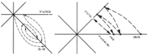
If we modify the rewards slightly to be ( r 1 , r2) (10, -7.8) then the true value function v· = (10 ~, ~ ) is no longer in 1i. The best representation of V* is V1£ = II1i V* = (10~ , 0) . If we start from (0, 0) as above, we will again reach a suboptimal fixed point around (5, -5) . How­ ever, starting from V 0 = (30, 0) (or even V0 = (15 , 0)) the result of repeated applications of II1i T as shown in Fig­ ure 1(b) displays a different type of failure- oscillation be­ tween points approaching (7 .5, 7 .5) and (16 , 0) . As in the pre­ vious example, IIV1£ - V*ll ,- is small, so the relative error bound is large.

4 The Bridge Algorithm

We begin with a high level description of the algorithm (de­ tails are in the Appendix). This is followed by the convergence results and another look at the examples from the pre­ vious section.

The main algorithm Bridge ValueDet, determines the value function within some error bound by making repeated calls to BridgeStep. We will now describe the first invoca­ tion of BridgeStep.

Metaphorically it consists of throwing a bridge across the treacherous terrain that is the hypothesis class 1i, towards a point on the far side of the optimal solution. If the bridge lands somewhere close to where we aimed it, we will be able to walk along it in a productive direction (achieve a contrac­ tion). If the bridge lands far from our target, then we know that there isn't any 1i-expressible value function near our target on which the bridge could have landed (hence an error bound). This is made precise by Lemma 2 in the next section.

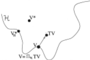
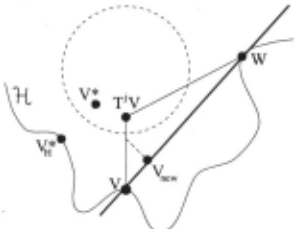
We are given an old approximation V from which we try to create a better approximation V n ew. We basically have two tools to work with: T and II1i. As can be seen in Figure2 (and in the example in the previous section), if we combine these two operators in the standard way, V n ew = II1iTV, we can get stuck in a local minimum. We will instead use them more creatively to guarantee progress or establish an error bound.

We begin by using not T but rather T i where j is deter­ mined by the main algorithm BridgeValueDet before it calls BridgeStep. We can then ask the question, given we know where V and TiV are, what does that tell us about the location of V*? It turns out that v· is restricted to lie in some hypersphere whose position can be defined in terms of the po­ sitions of V and TiV. This is made precise by Lemma 1 in the next section. The hypersphere is depicted in Figure 3 and as required, v· lies inside it.

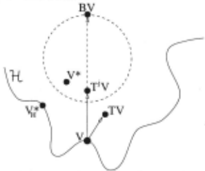
We now define a new operator B based on Ti and the iden­ tity operator I.

B simply amplifies the Bellman residual by a factor of 1 _! 11 · As can be seen in Figure 3, BV is the point on the far side of the hypersphere from V. This operator is what we use to throw a bridge. We aim the bridge for BV, which is beyond anywhere where our goal might be, i.e.the true value function lies somewhere between V and BV. The motivation for us­ ing B is in a sense to jump over all local minima between V and V*.

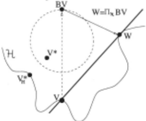
Ideally we would be able to represent BV Gust as in the standard approach we would want to represent TV) but this function is most likely not in our class of representable func­ tions. Therefore we must apply the operator II1l to map it into 1i. The result, W = II1lBV E 1i, is shown in Figure4. The bridge is supported by V and W and is shown as a line be­ tween them. In summary we throw the bridge aiming for BV, but II1l determines the point W on which it actually lands.

In practice we perform the mapping II1l by generating sam­ ples from an appropriate distribution and passing them to a learning algorithm for 1i. In particular to compute II1lBV, we generate samples (x, y) according to the distribution:

The key feature of this distribution is that if a random variable Y has associated density P~ (-/x) then E[Y] = BV(x).

The final step is to walk along the bridge. The bridge is a line between V and W and our new approximation V new will be some point on this line (see Figure 5). This point is deter­ mined by projecting a point TJ S 1 of the way from V to Ti V onto the line, where TJ is a function of the input parameters. (We could just project Ti V, but using TJ is a refinement that yields a better guaranteed effective contraction factor.)

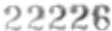
Thus the new approximation V new. which is not necessar­ ily in 1i, is a weighted average of the old approximation V and W E 1i. Calculating the weights (p and 1-p) in this average requires the ability to measure distance and risk. In particular we need to measure the distance between V and W and the risk of V and W with respect to the distribution Pj:i . These

2

,

three lengths (and T)) determine the relative position of v new with respect to V and W (See Figure 5). In practice we es­ timate the true risk with the empirical risk [Haussler, 1992], which we calculate using samples drawn from the distribution Pf~:

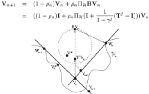
We have just described a single invocation of BridgeStep that represents the first iteration of the main algorithm. Each iteration builds a new bridge based on the previous one, so a generic iteration would begin with a V that was the V new of the previous iteration (see Figure 6). In particular, the input V of a generic iteration is not in 1i, but is rather a linear com­ bination of the initial approximation V 0 and all previous W functions. Thus the final result is a tall weighted tree whose leaves are in 1i. If we insist on a final result that is in 1i, then we can apply a final ITt£ mapping at the very end.

Just as the standard TD algorithm was summarized as V n + 1 = IItlTV n· the Bridge algorithm can be essentially summarized as

4.1 Convergence of the Bridge algorithm

We will state the main convergence theorem for the Bridge al­ gorithm, but space limitations allow us to state only the two most important Lemmas used in the proof. We begin with a very useful observation about the geometric relationship be­ tween V, TV and V* .

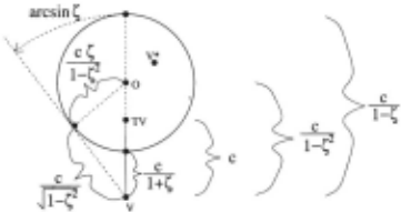
Lemma 1 Let A be a contraction with contraction factor ( under some norm. Let V* be the fixed point of A. For any pointY let 0 = V + 1 !e (AV- V). Then,

In words, given the positions of V and AV, let c = I!AV :..._VII. Then we know that the position of V* has to be on or inside the hypersphere of radius 1 ~12 centered at 0 (see Figure 7). This hypersphere is simply the set of points that are at least a factor of (closer to AV than to V. Note that the dis­ tance from V to the furthest point on the hypersphere is 1 ~(.

We apply Lemma 1 using Ti for A and lj for(. This de­ fines a hypersphere inside of which the true value function must lie. Lemma 1 is used mainly to prove Lemma 2, which characterizes the behavior of BridgeS tep and provides most of the meat of the convergence proof.

Lemma 2 Given an approximation V and parameters a > 0 and j 2 1, BridgeStep(V, a , j) returns a new approximation V new that satisfies at least one of the following two con­ ditions, where the error bound "' = err Bound( a, 1, j) is defined in the Appendix

Intuitively, if the bridge lands close to where we aimed it, we will achieve a contraction towards the goal. If the bridge lands far away, we will prove a relative error bound for the result. The key quantity that determines which of these two events happens, is the angle B formed between the bridge and the line from V to BV. If W = IIHBV is close to BV, then B will be small, the bridge will lie close to the hyper­ sphere, and we will be able to walk along the bridge and make progress. If instead W is far from BV, then B will be large and walking along the bridge will not take us closer to the goal, but we will be able to prove that we are already close enough.

Figure 8 shows the case where the angle B is small. As de­ scribed previously, the small hypersphere represents the set of points that are at least a factor of lj closer to TJV than they are to V. This follows from applying Lemma 1 to the operator TJ. Now think of BridgeStep as an operator that takes V and returns V new, and ask the question, what set of points are at least a factor of a (which is an input parame­ ter to BridgeStep) closer to V new than to V? Applying Lemma 1 to this question defines another, much larger hy­ persphere which is depicted in Figure 8 with center at 0 for the case B = arcsin a - arcsin /j. Note that this larger hy­ persphere completely contains the smaller hypersphere which contains v·. Thus V* also lies inside the larger hypersphere and so v new is at least a factor of a closer to v· than v is. This holds forB = arcsin a - arcsin /j. If B is smaller than this, the achieved contraction is even better.

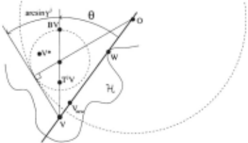
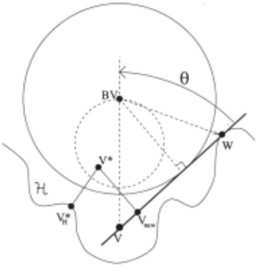
Figure 9 shows the case where the angle B is large. B is large when it is not possible to find a hypothesis in 1{ close to BV. In fact we choose W = IIHBV to be the closest such hy­ pothesis, so the rest of 1{ must lie further away. In particular 1{ must lie completely outside the big hypersphere depicted in Figure 9 with center at BV, for otherwise W would not be the closest hypothesis to BV. Furthermore we know that V* must lie on or inside the small hypersphere in Figure 9. Thus there is a separation between v· and 1{ and this separation allows us to prove, for any possible position of v·, an upper bound on the relative error ll~vr-~':; 1 1~w It should be noted that in general we do not know and we cannot measure B to determine which of the two conditions of Lemma 2 V new satisfies. We only know that it satisfies at least one of them.

By Lemma 2, if V already satisfies the relative error bound then so will v new. because if v new achieves a contraction over V, its error decreases. Thus each successive approxima­ tion is better than the one before, until we achieve the relative error bound from which point every subsequent approxima­ tion will also achieve that bound.

We now give the main result, which is guaranteed conver­ gence to a relative or absolute error bound. Moreover, the maximum number of invocations of BridgeStep, and thus the maximum number of hypotheses in the linear combina­ tion, can be specified.

Theorem 1 Let 11 > 1 and <o > 0 be the desired relative and absolute error bounds respectively. Let N be an upper bound on the desired number of iterations. Then the algorithm BridgeVa1ueDet(11, <o, N) produces an approximation V, consisting of a linear combination of at most N + 1 hypotheses from 1{, that satisfies at least one of either the relative error

bound 11 or the absolute error bound <a:

The proof of the theorem follows directly from Lemma 2; rewards are bounded, so the true value function is bounded, so the absolute error of the initial approximation can be bounded. If all N iterations achieve a contraction, then the absolute er­ ror will be smaller than requested. If at least one of the itera­ tions failed to achieve a contraction, then it achieved a relative error bound and all subsequent iterations, including the last one, will achieve the requested relative error bound. Again, since we do not know which of the two conditions of Lemma 2

each i~eration satisfies, we do not know whether the final an­ swer V satisfies the relative or the absolute error bound. We know only that it satisfies at least one of them.

Corollary 1 Let 11, fo and N be as defined in Theorem 1. Let V = Bridge ValueDet(11, fo, N ), a linear combination of hyp_otheses from 1l. Then v 1i = n1i V, the result of map­ ping V back into 1l, satisfies at least one of either the relative error bound 211 + 1 or absolute error bound fo (2 + ~ ).

4.2 The Examples Revisited

We now reconsider the examples from Section 3. The main algorithm Bridge ValueDet takes parameters 11 , fo, and N, from which it computes the number of lookahead steps j to use to achieve the requested error bounds. Also for each it­ eration, it chooses a parameter an which determines the con­ traction factor achieved or relative error bound established for that iteration. These two parameters, j and an, are passed to BridgeStep at each iteration. In this section, we exam­ ine the effect of repeated applications of BridgeStep, using j = 3 and a = .99 for every iteration.

For the first example, with initial V 0 = (0, 0), the results of repeated applications of BridgeSte p are shown in Fig­ ure lO(a). Because for this example IIV1£- V *ll 7r = 0 (i .e. the true value function is in 1£), the relative error bound is al­ ways infinite. Therefore, by Lemma 2, every step achieves at least a contraction a and so the algorithm converges to the true value function .

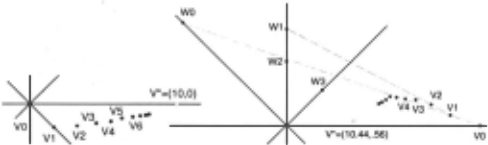
For the second example, with V 0 = (30, 0) , the results of repeated applications of BridgeStep are shown in Fig­ ure 10(b). Looking at the first step more closely, TiV0 = (10.2, 10.6),BVo = (-10.7,21.7)andWo = ll1iBVo = ( -16.2, 16.2). The dotted line between V 0 and W 0 is the bridge. V 1 , being a weighted average ofV0 and W 0 , lies on this bridge. Similarly, V 2 lies on the bridge between V 1 and w1.

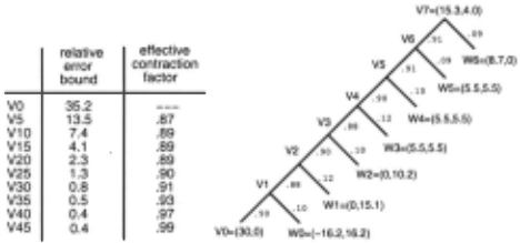
Figure ll(a) demonstrates Lemma 2 on every fifth appli­ cation of BridgeStep. In particular, note that the effective contraction factor only exceeds a after the desired relative er­ ror bound err Bound( a , 1, j) = 4.3 has been achieved. In fact on this example, the algorithm performs far better than the theory guarantees. Figure 11 (b) shows the weights of the averages and the structure of the resulting linear combination after 7 steps.

5 Extensions

It is possible to extend the algorithm in many ways. In partic­ ular relying on an exact, agnostic learning operator TTH is not practical. Here we briefly discuss the use of two other learning operators and we hope in the future to consider others still.

5.1 PAC(E 1 8) learning

Most significantly we have extended our algorithm to the case where the learning step n1i cannot be done exactly but is instead a PAC learning step ll~ 6 (see [Papavassiliou and Rus­ sell, 1998]). We actually use the same f and J for every iter­ ation, so the learning step n f,o has the same complexity for every iteration. This is sim;fe but most likely not optimal. One appealing aspect of considering PAC agnostic learning is the potential availability of sample complexity results based on some measure of the complexity of 1l. Unfortunately it is necessary to learn and estimate risk under the stationary distri­ bution of the Markov chain. Simply running the chain to gen­ erate samples will only generate them correctly in the steady­ state limit. Therefore computing sample complexity results for the risk estimation and agnostic learning steps requires ex­ tending the current state of the theory to the case where sam­ ples are generated from a Markov chain, rather than i.i .d. One would expect the sample complexity to depend on the mixing time of the Markov chain and the variance of the sample dis­ tribution. The form of these theorems will also determine the extent to which samples can be reused between the different risk estimation steps within an iteration or even across itera­ tions.

5.2 Suboptimallearning

Previous algorithms for this problem have been shown to con­ verge for learning operators n1i that are non-expansions

The convergence results for Bridge hold for learning operators that perform agnostic learning. Unfortunately there is a gen­ erallack of useful agnostic learning algorithms (the risk mini­ mization step is typically intractable), so it would be beneficial to extend the results to learning systems that are not optimal.

It is possible to weaken the conditions on the learning op­ erator and give convergence results for Bridge that hold when n1i satisfies the banana-fudge condition

for some nondecreasing functions k 1 > 0 and k2. The only modification necessary to Bridge is to includek1 and k2 in the calculation of the relative error bound err Bound( a,/, j). Note that for k 1 ( z) = 1 and k2 ( z) = z, this condition re­ duces to

which is in fact the property of agnostic learning that is used to derive the results in this paper.

Intuitively, the nonexpansion condition for n1i requires that two points that are close to each other, are mapped close to each other. The banana-fudge condition requires that two points that are close to each other, are mapped a similar dis­ tance away, but they can be mapped in opposite directions and so end up very far from each other. The banana-fudge con­ dition is obviously the weaker one, requiring only similarity in level of success and not similarity in outcome. It disal­ lows the case where one function is learned very well, but an­ other function very close to the first is learned very poorly. We are currently searching for learning algorithms that satisfy the banana-fudge condition, but unfortunately it seems most com­ mon practical learning algorithms do not.

6 Other Approaches

We briefly discuss other known alternatives to Bridge as well as mention some of the new directions one might consider.

6.1 Alternatives

If 1l is convex and IT11 is the agnostic learning operator, then IT11 is a nonexpansion and V n+1 = II11TV n con­ verges. For nonconvex 1l, an alternative approach to Bridge is to PAC-agnostically learn the convex hull of 1l using IT11 at each iteration [Lee et al., 1995]. The resulting iterated procedure V n +1 = I1convex -hu11(1i ) TV n converges since I1convex -hu11(1i ) is a nonexpansion. Unfortunately, this algo­ rithm requires many more agnostic learning steps per iteration than seems practical.

A noniterative method that returns the optimal answer is to reduce the value determination problem to a single instance of supervised learning by using the operator T 00 (otherwise known as TD(.A = 1)). It does unlimited lookahead, has con­ traction factor 7 00 = 0 and so it generates v· after just one it­ eration. Looked at another way, thedistributionPJ:"oo (·lx) has mean V*(x) and so II11T 00 V = V7£. Unfortunately there is empirical evidence that suggests the sample distribution PJ:"oo is very hard to learn and requires very many samples (perhaps because it can have high variance).

Strictly speaking, it is not necessary to backup values beyond the f-horizon which is log_,. €1 1 --y). Even this, however, may yield sample distributions with.too much variance for practical use, although it is offset by the need to perform only a single learning step.

Finally it may be possible, using Lemma 1, to establish convergence rates and error bounds for the iterated procedure V n+1 = II-~Tmv n where m is less than the f-horizon. However, m would probably have to be much larger than j, the number of lookahead steps used by Bridge, and so again we would expect bad sample complexity.

6.2 New Directions

There are many ways in which the basic tools used in con­ structing this algorithm might be used in constructing more powerful methods. Specifically the geometric relationship be­ tween V, TV, and v· established in Lemma 1 is very use­ ful in ( 1) providing geometric intuition to design new methods and (2) proving performance guarantees for these methods.

One can think of many different ways to throw a bridge and many different kinds of bridges to throw. For example, we es­ tablish W, the other end of the bridge by learning the point V + 1 _\ 1 (TiV- V). This choice is rather arbitrary, picked to simplify the error bound analysis. One might try instead learning a point further or a little closer to V.

Once we establish W, we throw a one-dimensional, linear bridge from V toW and learn a point close to TiV on this line (learning is equivalent to projection in linear hypothesis classes). One might try establishing more than two points with which to support the bridge. For example, given V and after establishing W (1 ), we could try establishing W (2) by learn­ ing a point strategically located far from both V and W(1) on the other side of the hypersphere defined by Lemma 1. Then we could throw a two-dimensional, planar bridge across these three points and project TJV (or a point close by) onto this plane. We can continue in this way, considering methods that establish W(1) , ... , W(n) and use ann-dimensional hyper­ plane to learn TJV. In the logical limit this method looks like a local version of [Lee et al., 1995] which learns the full convex hull. It is local in that it only closes under weighted averaging those points of 1l that are closest to some point of the hypersphere defined by Lemma 1. Our current method which only uses one-dimensional bridges is effectively a light version of these convex-hull methods, in that before learning TJV it closes under linear combinations only two points from 1l, namely V and W.

7 Conclusion

We have developed a method that reduces the value determi­ nation problem to the agnostic learning problem. Requesting that our algorithm halt in fewer iterations or with better er­ ror bounds pushes more of the complexity into the learning step and in the limit effectively forces it to consider infinite lookahead which is T 00 . Similarly, if we were to extend our algorithm to use more and more supports for the bridge, we suspect it would approximate the performance of the convex hull learning algorithm. Thus our method can be thought of as a more versatile and hopefully more efficient alternative to these aggressive methods.

The key features that characterize our approach are ( 1) the complication of learning is abstracted into a learning operator IT1f, (2) we use a new operator B rather than being restricted to the backup operator T, (3) we form linear combinations of hypotheses from a class 1l rather than being limited to just 1l, and (4) we use Lemma 1 to prove convergence and error bound results. These techniques can be applied or modified to develop endless variations on Bridge as well as completely new algorithms.

A big missing ingredient in justifying one method over an­ other is sample complexity. In particular, we do not know how sample complexity depends on the lookahead j, or, in the case ofiT~ 0 , how it depends on f, and so we cannot properly trade off these parameters to achieve the best performance.

Our results are stated for the problem of value determina­ tion, but they apply to any situation with an operator that is a contraction with respect to a norm defined by a samplable distribution. For the problem of value determination, the op­ erator is T , the one-step backup operator, and it is a con­ traction under the norm defined by the stationary distribution of the Markov chain. As stated previously, this distribution can only be sampled exactly in the steady-state limit, so im­ provements in the theory are necessary. Finally, a big hurdle to a practical, implementable algorithm is the lack of useful, well-behaved (agnostic or not) learning algorithms. By ap­ plying the techniques used in developing Bridge, we hope to bridge the gap between the available supervised learning al­ gorithms and those needed by theoretically justified reinforcement learning methods.