
Leave-One-Out Support Vector Machines
Proceedings of the Sixteenth International Joint Conference on Artificial Intelligence. Machine Learning. Pages 727-732.
© 1999 International Joint Conferences on Artificial Intelligence
Abstract
We present a new learning algorithm for pattern recognition inspired by a recent upper bound on leav e-o ne-out error [Jaakkola and Haussler, 1999] proved for Support Vector Machines (SVMs) [Vapnik, 1995; 1998]. The new approach directly minimizes the expression given by the bound in an attempt to minimize leave-one-out error. This gives a convex optimization problem which constructs a sparse linear classifier in feature space using the kernel technique. As such the algorithm possesses many of the same properties as SVMs. The main novelty of the algorithm is that apart from the choice of kernel, it is parameterless - the selection of the number of training errors is inherent in the algorithm and not chosen by an extra free parameter as in SVMs. First experiments using the method on benchmark datasets from the UCI repository show results similar to SVMs which have been tuned to have the best choice of parameter.
- [Cortes and Vapnik, 1995] Corinna Cortes and Vladimir Vapnik. Support Vector Networks. Machine Learning, 20:273-297, 1995.
- [Jaakkola and Haussler, 1999] Tommi S. Jaakkola and David Haussler. Probabilistic kernel regression mod- els. In Proceedings of the 1999 Conference on AI and Statistics. Morgan Kaufmann, 1999.
- [Osuna and Girosi, 1998] E. Osuna and F. Girosi. Re- ducing run-time complexity in SVMs. In Proceedings of the 14th Int'l Conf. on Pattern Recognition, Bris- bane, Australia, 1998.
- [Riitsch et al., 1998] Gunnar Riitsch, T. Onoda, and Klaus-Robert Muller. Soft margins for adaboost. Technical report, Royal Holloway, University of Lon- don, 1998. TR-98-21.
- [Scholkopf, 1997] Bernhard Scholkopf. Support Vector Learning. PhD thesis, Technische Universitii Berlin, Berlin, Germany, 1997.
- [Vapnik, 1995] Vladimir Vapnik. The Nature of Statis- tical Learning Theory. Springer-Verlag, New York, 1995.
- [Vapnik, 1998] Vladimir Vapnik. Statistical Learning Theory. John Wiley and Sons, New York, 1998.
References were extracted automatically from the PDF and may contain errors.
Full text extracted automatically from the PDF; figures, tables and equations may differ. The PDF is the version of record.
1 Introduction
Support Vector Machines (SVMs), motivated by mini mizing VC dimension, have proven to be very successful in classification learning [Vapnik, 1995; Scholkopf, 1997; Vapnik, 1998] . In this algorithm it turned out to be favourable to formulate the decision functions in terms of a symmetric, positive definite, and square integrable function k(·, ·) referred to as a kernel. The class of decision functions - also known as kernel classifiers [Jaakkola and Haussler, 1999] - is then given by
where training data Xi E IRN and labels Yi E { ± 1}. For simplicity we ignore classifiers which use an extra threshold term.
Recently, utilizing this particular type of decision rule (that each training point corresponds to one basis func tion) an upper bound on leave-one-out error for SVMs was proven [Jaakkola and Haussler, 1999]. This bound motivates the following new algorithm: find a decision rule of the form in Equation (1) that minimizes the bound. The paper is structured as follows: In Section 2 we first review the SVM algorithm. In Section 3 we de scribe the leave-one- out bound and the Leave-One-Out Support Vector Machine (LOOM) algorithm motivated by the bound. In Section 4 we reveal the relationship between SVMs and LOOMs and in Section 5 results of a comparison of LOOMs with SVMs on artificial and benchmark datasets from the UCI repository are pre sented. Finally, in Section 6 we summarize and discuss further directions.
2 Support Vector Machines
Support vector machines [Vapnik, 1995] aim to mini mize VC dimension by finding a hyperplane with mini mal norm that separates the training data mapped into a feature space :F via a nonlinear map ~ : JRN --+ :F. To construct such a hyperplane in the general case where one allows some training error one minimizes:
subject to
and then uses the decision rule:
The tractability of this algorithm depends on the di mensionality of :F. However, one can remove this depen dency by instead maximizing the dual form:
where, utilizing that
and that k(x,x') = (<ll(x) · <ll(x')), the decision rule is now in the form of Equation (1).
Alternatively, one can also use the primal dual formu lation of the SVM algorithm (from [Osuna and Girosi, 1998]) rather than the usual formulation, which we will describe because of its direct correlation to Leave- One Out SVMs. The SVM primal reformulation is the fol lowing: minimize
subject to
where one again uses a decision rule of the form in Equa tion (1).
3 Leave-One-Out Support Vector Machines
Support Vector Machines obtain sparse solutions that yield a direct assessment of generalization: leave-one-out error is bounded by the expected ratio of the number of non-zero coefficients to the number of training exam ples [Vapnik, 1995]. In [Jaakkola and Haussler, 1999) a measure of generalization error is derived for a class of classifiers which includes SVMs but can be applied to non-sparse solutions. The bound is as follows:
Theorem 1 For any training set of examples x; E IRN and labels y; E { ± 1}, for a SVM trained by maximiz ing Equation (6} the leave- one- out error estimate of the classifier is bounded by
where B( ·) is the step function.
This bound is slightly tighter than the classical SVM leave- one- out bound. This is easy to see when one con siders that all training points that have a; = 0 can not be leave-one-out errors in either bound. Vapnik's bound assumes all support vectors (all training points with a; > 0) are errors, whereas they only contribute as errors in Equation (11) if
In practice this means the bound is tighter for less sparse solutions.
Although the leave- one-out bound in Theorem 1 holds for Support Vector Machines the motivation behind SVMs is to minimize VC bounds via Structural Risk Minimization [Vapnik, 1995]. To this end, the term 'L a;aiYiYjk(x;, Xj) in Equation (8) attempts to min imize VC dimension. If we wish to construct classi fiers motivated by Theorem 1 (that directly attempt to achieve a low value of this expression) we need to con sider a different learning technique.
Theorem 1 motivates the following algorithm: directly minimize the expression in the bound. To do this, one in troduces slack variables following the standard approach in [Cortes and Vapnik, 1995; Vapnik, 1995) to give the following optimization problem: minimize
subject to
where one chooses a fixed constant for the margin to ensure non-zero solutions.
To make the optimization problem tractable, the smallest value for 6 for which we obtain a convex ob jective function is 6 = 1. This gives us a linear program ming problem, and, as in other kernel classifiers, one uses the decision rule given in Equation (1).
Note that Theorem 1 is no longer valid for this learn ing algorithm. Nevertheless, let us study the resulting method which we call a Leave- One- Out Support Vector Machine (LOOM).
4 Relationship to SVMs
In this section, we will describe the relationship between LOOMs and SVMs in three areas: the method of regu larization, the sparsity induced in the decision function and the margin loss employed in training.
4 .1 Regularization
The new technique appears to have no free regularization parameter. This should be compared with SVMs which control the amount of regularization with the free pa rameter C. For SVMs, in the case of C = oo one obtains a hard margin classifier with no training errors. In the case of noisy or linearly inseparable datasets 1 (through noise, outliers, o~ class overlap) one must accept some training error (by constructing a so called soft margin). To find the best choice of training error/margin tradeoff one must choose the appropriate value of C. In LOOMs a soft margin is automatically constructed. This occurs because the algorithm does not attempt to minimize the number of training errors - it minimizes the number of training points that are classified incorrectly even when they are removed from the linear combination that forms the decision rule. However, if one can classify a train ing point correctly when it is removed from the linear combination then it will always be classified correctly when it is placed back into the rule. This can be seen as ow;k(x;, x;) is always the same sign as y;, all train ing points are pushed towards the correct side of the decision boundary by their own component of the linear combination.
1 Here we refer to linear inseparability in feature space. Both SVMs and LOOM Machines are essentially linear classifiers.
4.2 Sparsity
Like Support Vector Machines, the solutions of the new algorithm can be sparse; that is, only some of the co efficients a;, i = 1, ... , e are non- zero (see Section 5.2 for computer simulations confirming this). As the coeffi cient of a training point does not contribute to its leave one- out error in constraint (13) the algorithm does not assign a non-zero value to the coefficient of a training point in order to correctly classify it. A training point has to be classified correctly by the training points of the same label that are close to it (in feature space), but the training point itself makes no contribution to its own classification.
4.3 Margin loss
Noting that
where f(x) is given in Equation (1), one can see that the new algorithm can be written as the following equivalent linear program: minimize
subject to
In this setting of the optimization problem it is easy to see that a training point Xi is linearly penalized for failing to obtain a margin of Pt(xi, Yi) 2': 1 + aik(xi, xi)· In SVMs, a training point Xi is linearly penalized for failing to obtain a margin of p 1 (xi, y;) 2': 1 (see Equation (9)). Thus the margin in SVMs is treated equivalently for each training pattern. In LOOMs, the larger the contribution the training point has to the decision rule (the larger the value of a;), the larger its margin must be. Thus, the LOOM algorithm, in contrast to SVMs controls the margin for each training point adaptively.
This method can be viewed in the following way: If a point <I>(xk) is an outlier (the values of k(xi,xk) to points <I>(xi) in its class are small and to points in the other class are large) then some ai, where Yi = Yk, in Equation (13) have to be large in order to classify <I>(xk) correctly. SVMs use the same margin for such points
<I>(x;) and they attempt to classify <I>(xk) correctly. In LOOMs the margin is automatically increased to 1 + aik(x;, x;) for these points and thus less attempt is made to correctly classify <I>(xk)· Thus the adaptive margin provides robustness. Moreover, it becomes clear that in LOOMs the points <I>(xk) which are representatives of clusters (centres) in feature space, i.e. those which have large values of k(x;, xk) to points in their class, will have non- zero ak.
5 Experiments
In this section we describe experiments comparing the new technique to SVMs. We first describe artificial data to visualize the techniques, and then present results on benchmark datasets.
5.1 Artificial Data
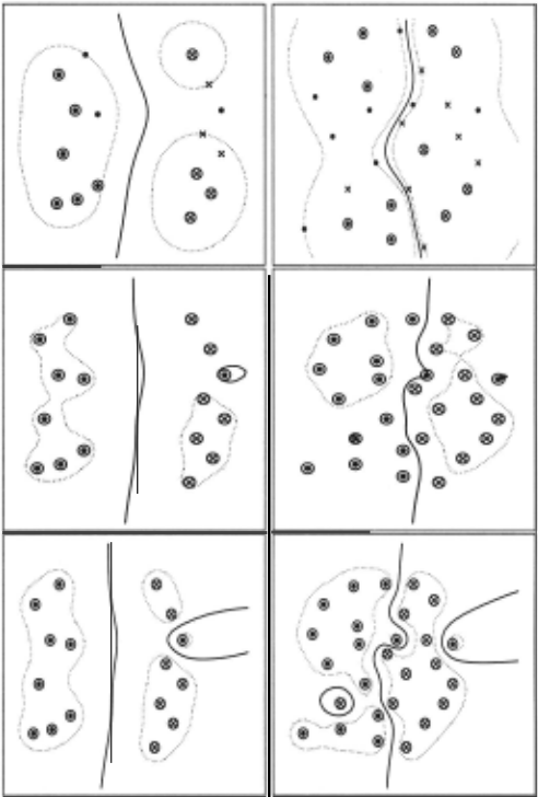
We first describe some toy two dimensional examples to illustrate how the new technique works. Figure 1 shows two artificially constructed training problems (left and right) with various solutions (top to bottom of the page). We fixed the kernel to be a radial basis function (RBF)
with A = 1 and then found the solution to the problems with Leave-One-Out Machines (LOOMs), which have no other free parameters, and with SVMs, for which one controls the soft margin with the free parameter C. The first solution (top of the page) for both training problems (left and right) is the solution given by LOOMs, and the other four solutions are SVMs with various choices of soft margin (parameter C).
In the first problem (left) the two classes (crosses and dots) are almost linearly separable apart from a single outlier (a dot). The automatic soft margin control of LOOMs constructs a classifier which incorrectly clas sifies the far right dot, assuming that it is an outlier. Thick lines represent the separating hyperplane and dot ted lines represent the size of margin. Support Vec tors (training points with a; > 0) are emphasized with rings. Note also the large margin of the LOOM classi fication. The Support Vector solutions (second picture from top downwards) have parameters C = 1 (middle) and C = 100 (bottom). Constructing a hard margin with C = 100 overfits with zero training error whilst with de creasing C the SVM solution tends towards a decision rule similar to the one found by LOOMs. Note, however, even with C = 1 the non-smoothness of the decision rule by examining the margin (dotted line). Moreover, the outlier here is still correctly classified.
In the second training problem (right), the two classes occupy opposite sides (horizontally) of the picture, but slightly overlap. In this case the data is only separa ble with a highly nonlinear decision rule, as reflected in the hard margin solution by an SVM with parame ter C = 100 (bottom right). Again, a reasonable choice of rule (C = 1, middle right picture) can be found by SVMs with the correct choice of free parameter. The (parameterless) decision constructed by the LOOM (top right) however provides a similar decision to the SVM with C = 1. Note again, the smoothness of the LOOM solution in comparison to the SVM one, even though they are similar.
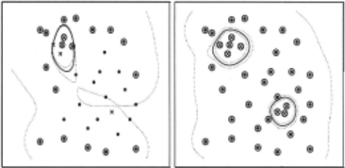
Finally, Figure 2 gives some insight into how the soft margin is chosen by LOOMs. A simple toy training set is again shown. The first picture (left) has a small cluster of crosses in the top left of the picture and a single cross in the bottom right of the picture. The other class (dots) is distributed almost evenly across the space. LOOMs construct a decision rule which treats the cross in the bottom right of the picture as an outlier. In the second picture (right) we have almost the same problem but near the single cross we add another two training points so there are now two clusters of crosses. Now the LOOM
solution is a decision rule with two clusters; because the single cross from the left hand picture now is close to other training points, it can be left out of the decision rule but still be classified correctly in the constraints (13). When a training point is not close (in feature space) to any other points in the same class it is considered an outlier.
5.2 Benchmark Datasets
We conducted computer simulations using 6 artificial and real world datasets from the UCI, DELVE and STATLOG benchmark repositories, following the same experimental setup as in [Riitsch et al., 1998]. The au thors of this article also provide a website to obtain the data 2 . Briefly, the setup is as follows: the performance of a classifier is measured by its average error over one hundred partitions of the datasets into training and test ing sets. Free parameter(s) in the learning algorithm are chosen as the median value of the best model chosen by cross validation of the first five training datasets.
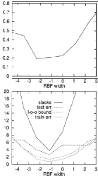
Table 1 compares percentage test error of LOOMs to AdaBoost (AB), Regularized AdaBoost (ABR) and SVMs which are all known to be excellent classifiers 3 . The competitiveness of LOOMs to SVMs and ABR (which both have a soft margin control parameter) is remarkable considering LOOMs have no free parame ter. This indicates that the soft margin automatically selected by LOOMs is close to optimal. AdaBoost loses Finally, to show the behaviour of the algorithm we give two plots in Figure 3. The top graph shows the fraction of training points that have non-zero coefficients (SVs) plotted against log(A) (REF width) on the thy roid dataset . Here, one can see the sparsity of the de cision rule ( cf. Equation (1)), the sparseness of which depends on the chosen value of A. The bottom graph shows the number of training and test errors (train err and test err) , the value of .z::::;=l ~i (slacks) and the value of the bound given in Theorem 1 ( l-o-o bound). One can see the training and test error (and the bound) closely match which would be natural for an algorithm which minimized leave-one-out error. The minimum of all four plots is roughly at log(A) = -1, indicating one could perform model selection using one of the known expres sions. Note also that for a reasonable range of different RBF widths the test error is roughly the same, indicating the automatic soft margin control overcomes overfitting problems. Moreover, the values of A which give the best generalization error also give the most sparse classifiers.
2 http: / /svm.first.gmd.de/ ~raetsch/ data/benchmarks.htm. The datasets have been pre-processed to have zero mean and standard deviation one, and the exact one hundred splits of training and testing sets used in the author's experiments can be obtained.
3 The results for AB, ABR and SVMs were obtained by Riietsch, et al.
| AB | ABR | SVM | LOOM | |
|---|---|---|---|---|
| Banana | 12.3 | 10.9 | 11.5 | 10.6 |
| B. Cancer | 30.4 | 26.5 | 26.0 | 26.3 |
| Diabetes | 26.5 | 23.9 | 23.5 | 23.4 |
| Heart | 20.3 | 16.6 | 16.0 | 16.6 |
| Thyroid | 4.4 | 4.4 | 4.8 | 5.0 |
| Titanic | 22.6 | 22.6 | 22.4 | 22.7 |
Table 1: Comparison of percentage test error of Ad aBoost (AB), Regularized AdaBoost (ABn), Support Vector Machines (SVMs) and Leave-One-Out Machines (LOOMs) on 6 datasets.
6 Discussion
In this article, motivated by. a bound on leave-one-out error for kernel classifiers, we presented a new learning algorithm for solving pattern recognition problems. The robustness of the approach, despite having no regular ization parameter, can be understood in terms of the bound (one must classify points correctly without their own basis function) , in terms of margin (see Section 4.3), and through empirical study. We would also like to point out that if one constructs a kernel matrix Kij = k(xi, xi) then the regularization technique employed is to set the diagonal of the matrix to zero, which suggests that one can control regularization through control of the ridge, as in regression techniques.
Acknowledgments We would like to thank Vladimir Vapnik, Ralf Herbrich and Alex Gammerman for their help with this work. We also thank the ESPRC for pro viding financial support through grant GR/L35812.
fll
> (/)
@inproceedings{ijcai1999p104,
  title     = {Leave-One-Out Support Vector Machines},
  author    = {Weston, Jason},
  booktitle = {Proceedings of the Sixteenth International Joint Conference on
               Artificial Intelligence, {IJCAI-99}},
  publisher = {International Joint Conferences on Artificial Intelligence},
  editor    = {Thomas Dean},
  pages     = {727--732},
  year      = {1999},
  note      = {Machine Learning},
  url       = {https://ijcai.org/proceedings/1999/104},
}
TY - CPAPER TI - Leave-One-Out Support Vector Machines AU - Weston, Jason T2 - Proceedings of the Sixteenth International Joint Conference on Artificial Intelligence, IJCAI-99 PB - International Joint Conferences on Artificial Intelligence PY - 1999 SP - 727 EP - 732 UR - https://ijcai.org/proceedings/1999/104 ER -Copied
Machine-readable versions of this paper, for tools and AI agents:





