
Semantically Guided Theorem Proving for Diagnosis Applications
Proceedings of the Fifteenth International Joint Conference on Artificial Intelligence. Diagnosis and Qualitative Reasoning. Pages 460-464.
© 1997 International Joint Conferences on Artificial Intelligence
Abstract
In this paper we. demonstrate how general purpose automated theorem proving techniques can be used to solve realistic model-based diagnosis problems. For this we modify a model generating tableau calculus such that a model of a correctly behaving device can be used to guide the search for minimal diagnoses. Our experiments show that our general approach is competitive with specialized diagnosis systems.
- I. P. Baumgartner, U. Furbach, and I. Niemela. Hyper Tableaux. In lELIA 96. European Workshop on Logic in AI, Springer, LNCS, 1996.
- F. Bry and A. Yahya. Minimal Model Generation with Positive Unit Hyper-Resolution Tableaux. In P. Moscato, U. Moscato, D. Mundici, and M. Omaghi, editors, Theorem Proving with Analytic Tableaux and Related Methods, volume 1071 of Lec- ture Notes in Artificial Intelligence, pages 143-159. Springer, 1996.
- C. Chang and R. Lee. Symbolic Logic and Mechanical Theorem Proving. Academic Press, 1973.
- H. Chu and D. Plaisted. Semantically Guided First-Order The- orem Proving using Hyper-Linking. In A. Bundy, editor, Au- tomated Deduction-CADE 12, LNAI 814, pages 192-206, Nancy, France, June 1994. Springer-Verlag.
- P. Frohlich and W. Nejdl. A model-based reasoning approach to circumscription. In Proceedings of the 12th European Con- ference on Artificial Intelligence, 1996.
- H. Ganzinger, C. Meyer, and C. Weidenbach. Soft Typing for Ordered Resolution. Unpublished, 1996.
- The ISCAS-85 Benchmarks. http: I /www. cbl . ncsu . edu/ www/CBLJDocs/iscas85.html, 1985. Link
- R. Manthey and F. Bry. SATCHMO: a theorem prover im- plemented in Prolog. In Proc. 9th CADE. Argonnee, Illinois, Springer LNCS, 1988.
- W. Nejdl and P. Frohlich. Minimal model semantics for diagno- sis -techniques and first benchmarks. In Seventh International Workshop on Principles of Diagnosis, Val Morin, Canada, Oct. 1996.
- R. Reiter. A theory of diagnosis from first principles. Artificial Intelligence, 32:57-95, 1987.
References were extracted automatically from the PDF and may contain errors.
Full text extracted automatically from the PDF; figures, tables and equations may differ. The PDF is the version of record.
1 Introduction
In this paper we will demonstrate that model generation theo rem proving is very well suited for solving consistency-based diagnosis tasks. More precisely, we want to emphasize two aspects:
- Theorem proving techniques are very well applicable to realistic diagnosis problems, as they are contained in di agnosis benchmark suites.
- ii) Semantic information from a specific domain, can be used to significantly improve performance of a theorem prover.
According to Reiter ([10]) a simulation model of the tech nical device under consideration is constructed and is used to predict its normal behavior. By comparing this prediction with the actual behavior it is possible to derive a diagnosis.
This work was motivated by the study of the diagnosis sys tem DRUM-2 [5; 9] . The basic idea is to start with anini tial model of a correctly functioning device. This model is revised, whenever the actual observations differ from the pre dicted behavior.
We will use a proof procedure, which is an implementation of the hyper tableaux calculus presented in [1]. We adapt the idea from DRUM-2 to this tableaux calculus, which yields semantic hyper tableaux. The resulting system approximates the efficiency of the DRUM-2 system.
The use of semantics within theorem proving procedures have been proposed before. There is the well-known con cept of semantic resolution ([3]) and, more recently, there are approaches by Plaisted ([4] and Ganzinger ([6]). Plaisted is arguing strongly for the need of giving semantic information for controlling the generation of clauses in his instance-based
Ulrich Furbach
Univ. Koblenz, Inst. f. Informatik
uliCOinfko.uni-koblenz.de
proof procedures, like hyper-linking. Ganzinger and his co workers are presenting an approach where orderings are used to construct models of clause sets. Indeed, they even relate their approach to SATCHMO-like theorem proving, which is an instance of the hyper tableau calculus. However, the semantics have to be given by orderings or alternatively, by Horn subsets of the set of clauses. In cases where the initially given semantics is not compatible with orderings or is not ex pressible by Horn subsets it is unclear how to proceed. We will show, that in the case of diagnosis an initial semantics, which is naturally given by a model of the correct behavior of the device under consideration, can improve performance significantly. Our proof procedure does not impose any re strictions on these initial models.
We assume that the reader is familiar with the basic con cepts of propositional logic. Clauses, i.e. multisets ofliterals, are usually written as the disjunction A1 V · · · V Am V ·E1 V · · · V ·En or as an implication A1, ... , Am +- E1, ... , En (m 2: 0, n 2: 0). With L we denote the complement of a literal L. Two literals Land K are complementary ifL = K.
2 Model-Based Diagnosis
In model-based diagnosis [10] a simulation model of the de vice under consideration is used to predict its normal behav ior, given the observed input parameters. This approach uses an logical description of the device, called the system descrip tion (SD), formalized by a set of first-order formulas. The system description consists of a set of axioms characteriz ing the behavior of system components of certain .types. The topology is modeled separately by a set of facts. The diag nostic problem is described by system description SD, a set COMP of components and a set OES of observations (log ical facts). With each component we associate a behavioral mode: Mode(c, Ok) means that component cis behaving correctly, while Mode( c, A b) (abbreviated by Ab( c)) denotes that c is faulty.
Definition 2.1 (Reiter 87) A Diagnosis of (SD, COMP, OES) is a set ~ ~ COMP, such that SD U OES U {Mode(c,Ab)lc E ~} U {·Mode(c,Ab)lc E COMP- ~} is consistent. ~is called a Minimal Diagnosis, iff it is the minimal set (wrt. ~)with this property. D
The set of all minimal diagnoses can be large for complex technical devices. Therefore, stronger criteria than minimal-
Wolfgang Nejdl
Unive.rsWit Hannover
nejdlCOkbs.uni-hannover.de ity are often used to further discriminate among the minimal diagnoses. These criteria are usually based on the probability or cardinality of diagnoses. In the remainder of this paper we will use restrictions on the cardinality of diagnoses. We say that a diagnosis satisfies the n-fault assumption iff IL11 :::; n. Other minimality criteria which prefer e.g. more probable di agnoses are conceivable as well, but are not treated in the present paper.
A widely used example of the n-fault assumption is the !-fault assumption or Single Fault Assumption. Many spe cialized systems for technical diagnosis have the Single Fault Assumption implicit and are unable to handle multiple faults.
In model-based diagnosis systems the Single Fault Assumption can be acti vated explicitly in order to provide more discrimination among diagnoses and to speed up the diagnosis process.
As a running example consider the sim ple digital circuit on the right consisting of an or-gate (or1) and two inverters (inv1 and inv2). The system description SD is given by the following propositional clauses: 1 ·
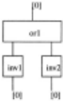
OR! : ab( orl ), high( orl, il ), high( orl, i2) f- high( orl , o) ab( orl ), high( orl , o) f- high( orl , il) ab( orl ), high( orl, o) f- high( orl, i2) INV I: ab( invl) f- high( invl, o ), high( invl, i) ab(invl),high(invl ,i),high(invl ,o) fINV2: ab(inv2) f- high(inv2 , o),high(inv2 , i) ab( inv2), high( inv2 , i) , high( inv2, o) fhigh( orl, il) f- high( invl, o) high( orl, i2) f- high( inv2, o) high( invl, o) f- high( orl , il) high( inv2 , o) f- high( orl, i2)We observe that both inputs of the circuit have low volt age and the output also has low voltage, i.e. the clause set of OBS is given by { f- high( inv1, i), +- high( inv2, i), t high( or1 , o) }.
The expected behavior of the circuit given that both inputs are low would be high voltage at the outputs of both inverters and consequently high voltage at the output of the or-gate. This model of the correctly functioning device, namely 10 = {high( inv1, o ) , high( inv2, o), high( or1, i1 ), high( or1, i2), high (or 1 , o)} , can be computed very efficiently even for large devices by domain-specific tools, e.g. circuit simulators.
1 These formulas can be obtained by instantiating a first or der description of the gate functions with the structural infor mation. For instance, the clauses for the OR I gate stem from the formula VOR_gd.te : ( ·ab( OR_gate)-+ (high( OR_gate, o) t-t (high( OR_gate , il) V high( OR_gate, i2) )) )
3 Hyper Tableaux Calculus
In [ 1] a variant of clausal normal form tableaux called "hyper tableaux" is introduced. We briefly recall the ground version here.
From now on S always denotes a finite ground clause set, and I: denotes its signature, i.e. the set of all predicate sym bols occurring in it. We consider finite ordered trees T where the nodes, except the root node, are labeled with literals. In the following we will represent a branch b in T by the se quence b = L 1 , ... , Ln ( n 2: 0) of its literal labels, where L 1 labels an immediate successor of the root node, and Ln la bels the leaf of b. The branch b is called regular iff L; =j:. L1 for 1 :::; i ,j :::; n and i =j:. j, otherwise it is called irregular. The tree T is regular iff every of its branches is regular, otherwise it is irregular. The set of branch literals of b is lit( b) = { L 1 , ... Ln} . For brevity, we will write expressions like A E b instead of A E lit( b) . In order to memorize the fact that a branch contains a contradiction, we allow to label a branch as either open or closed. A tableau is closed if each of its branches is closed, otherwise it is open.
Definition 3.1 (Hyper tableau) A literal set is called in consistent iff it contains a pair of complementary literals, oth erwise it is called consistent. Hyper tableaux for S are induc tively defined as follows:
Initialization step: The empty tree, consisting of the root node only, is a hyper tableau for S. Its single branch is marked as "open".
Hyper extension step: If (I) T is an open hyper tableau for S with open branch b, and (2) C = A1, ... ,Am+- B1, .. . ,En is a clause from S ( m 2: 0, n 2: 0), called extending clause in this context, and (3) { B 1 , ... , Bn} ~ b (equivalently, we say that C is applicable to b) then the tree T' is a hyper tableau for S, where T' is obtained from T by extension of b by C: replace b in T by the new branches
and then mark every inconsistent new branch as "closed", and the other new branches as "open". We say that a branch b is finished iff it is either closed, or else whenever C is applica ble to b, then extension of b by C yields some irregular new branch. D
The applicability condition of an extension expresses thiJ.t all body literals have to be satisfied by the branch to be extended (like in hyper resolution). From now on we consider only regular hyper tableaux. This restriction guarantees that for finite clause sets no branch can be extended infinitely often.
Definition 3.2 (Branch Semantics) As usual, we represent an interpretation I for given domain I: as the set {A E I: I I(A) =true, A atom}. Minimality of interpretations is de fined via set-inclusion.
Given a tableau with consistent branch b. The branch b is mapped to the interpretation [bh :=lit( b)+, where lit( b)+= {A E lit( b) I A is a positive literal } . Usually, we write [b] instead of [ b h and let 1: be given by the context. D
Figure 1 contains a hyper tableau for the clause set from our running example. Each open branch for the clause set SD U OBS corresponds to a partial model. The high lighted model can be understood as an attempt to construct a model for the whole clause set, without assuming unnecessary ab-predicates. Only for
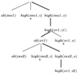
making the clauses from OR1 true is it necessary to include ab (or 1) into the model. high ( or1 , o) cannot be assumed, as this contradicts the observation +- high (or 1 , o).
A refutational completeness result for hyper tableaux was given in [1]. For our purposes of computing diagnosis (i.e. models), however, we need a (stronger) model completeness result:
Theorem 3.3 (Model Completeness of Hyper Tableaux.) Let T be a hyper tableau for S such that every open branch is finished. Then, for every minimal model I of S there is an open branch b in T such that I = [ b] .
This theorem enables us to compute in particular minimal di agnosis by simply collecting all Ab-literals along [b], be cause every minimal diagnosis must be contained in some minimal model of S.
3.1 Lessons from the Specialized Diagnosis System DRUM-2
In order to make the generation of models efficient enough for the large benchmark circuits used in this paper, additional knowledge has to be used to guide this model generation. This is done by starting from a model of the correct behav ior of the device SD and revising the model only where nec essary. This idea of a "semantically guided" model gener atio~ has been introduced first in the DRUM-2 system [5; 9]. The basic idea of DRUM-2 is to start with a model of the correct behavior of the device under consideration, i.e. with an interpretation I0 , such that I0 f= SD U { ·Ab( c)lc E COMP}. Then the system description SD is augmented by an observation of abnormal behavior OBS, such that the assumption that all components are working correctly is no longer valid. Thus, I0 is no model of SD U OBS, however it is used to guide the search for models of SD U OBS.
Note, that the initial model I 0 usually already takes into account a part of the observations which correspond to the inputs of the device under consideration. These input values are needed to simulate the correct behavior of the device. In our example, the initial model reflects the fact that the inputs ofthe inverters both have low voltage {I~ was given at the end of Section 2).
4 Formalizing the Diagnosis Task with Semantic Hyper Tableaux
In this section we discuss how to incorporate initial interpre tations into the calculus. Our first technique by cuts should be understood as the semantics of the approach; an efficient implementation by a compilation technique is presented af terwards.
4.1 Initial Interpretations via Cuts
The use of an initial interpretation can be approximated in the hyper tableau calculus by the introduction of an additional inference rule, the atomic cut rule.
Definition 4.1 The inference rule Atomic cut (with atom A) is given by: if
Tis an open hyper tableau for S with open branch b, then the literal tree T' is a hyper tableau for S, where T' is obtained from T by extension of b by A V ·A (cf. Def. 3.1). D
Note that in regular tableaux it cannot occur that a cut with atom A is applied, if either A or ·A is contained on the branch. As a consequence it is impossible to use the "same cut" twice on a branch.
We approximate initial interpretations by applying atomic cuts at the beginning of each hyper tableau:
Definition 4.2 An initial tableau for an interpretation Io is given by a regular tableau which is constructed by a applying atomic cuts with atoms from I 0 as long as possible. D
The branches of an initial tableau for an interpretation I 0 consist obviously of all inter pretations with atoms from Io . A part of the initial tableau for the initial interpretation I 0 given at the end of Section 2 is depicted in Figure 2. Note that the highlighted branch corre sponds to the highlighted part in Figure 1 (a negative literal
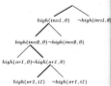
in an initial tableaux, such as ·high ( or1 , o), is represented implicitly in a hyper tableau as the absence of the comple mentary positive literal). If this branch is extended in succes sive hyper extension steps, the diagnosis ab (or 1), which was contained in the model from Figure 1 can be derived as well.
Definition 4.3 (Semantic Hyper Tableau - SHT) A se mantic hyper tableau for 10 and Sis a hyper tableau which is generated according to Definition 3.1, except that the empty tableau in the initialization step is replaced by an initial tableau for Io . D
It is easy to derive an open tableau starting from the initial tableau for I 0 in Figure 2, such that it contains the model from Figure I.
Proposition 4.4 (Model Completeness of SHT) Let T be a semantic hyper tableau for Io and S, such that every open branch is finished. Then, for every minimal model I of S there is an open branch bin T such that I= [b].
4.2 Initial Interpretations via Renaming
The just defined "semantical" account for initial interpreta tions via cut is unsuited for realistic examples. This is, be cause all the 2n - 1 possible deviations from the initial in terpretation will have to be investigated as well. Hence, in this section we introduce a compilation technique which im plements the deviation from the initial interpretation only by need.
Assume we have an initial interpretation Io = {a} and a clause set which contains b +-- and c +-- a 1\ b. By the only applicable atomic cut we get the initial tableau with two branches, name! y { a} and {-,a}. The first branch can be ex tended twice by an hyper extension step, yielding {a, b, c }. The second branch can be extended towards { ·a, b }. No more extension step is applicable to this tableau. Let Tcut be this tableau.
Let us now transform the clause set with respect to Io, such that every atom from ! 0 occurring in a clause is shifted to the other side of the +-- symbol and complemented. In our ex ample we get the clause c V ·a +--. b; the fact b +-- remains, because b is not in ! 0 · Using b +-- we construct a tableau consisting of the single branch { b }, which can be extended in an successive hyper step by using the renamed clause. We get a tableau consisting of two branches { b, c} and { b,-, a}. Let T be that tableau. Now, let us interpret a branch in T as usual, except that we set an atom from Io to true if its nega tion is not contained in the branch. Under this interpretation the branch { b, c} in T corresponds to the usual interpretation of {a , b, c} in Tcut· Likewise, the second branch { b, ·a} in Tcut corresponds to the second model in T.
Note that by this renaming we get tableaux where atoms from 10 occur only negatively on open branches; such cases just mean deviations from 10 . In contrast to the cut approach, these deviations are now brought into the tableau by need.
The following definition introduces the just described idea formally. Since we want to avoid unnecessary changes to the hyper calculus, a new predicate name neg_A instead of ·A will be used.
Definition 4.5 (!-transformation) Let C = L1 V · · · V Ln be a clause and I be a set of atoms. The I -transformation of C is the clause obtained from C by replacing every positive literal A with A E I by ·neg.A, and by replacing every nega tive literal ·A with A E I by neg.A. The I -transformation of S, written as 5 1 , is defined as the I -transformation of every clause inS. D
It is easy to see that every I -transformation preserves the models of a clause set, in the sense that every model for the non-transformed clause set constitutes a model for the trans formed clause set by setting neg_A to true iff A is false, for every A E I, and keeping the truth values for atoms outside of I . More formally we have:
Proposition 4.6 (Model Preservation of !-transformation)
For every interpretation J: J f= S iff rename1(J) f= 5 1 , where rename1(J)(neg.A) = J(A) iff A E J, and else rename1(J)(A) = J(A).
As explained informally above, the branch semantics of tableaux derived from a renamed, i.e. I -transformed clause set, is changed to assign true to every atom from I, unless its negation is on the branch. This is a formal definition:
The connection of semantic hyper tableaux to hyper tableaux and renaming is given by the next theorem.
Theorem 4. 7 Let T be a semantic hyper tableau for Sand I where every open branch is finished; Jet T 1 be a hyper tableau for the I -transformation of S where every open branch is fin ished. Then, for every open branch b 1 in T 1 there is an open branch bin T such [b 1 ] 1 = [b]. The converse does not hold.
The theorem tells us that with the renamed clause set we com pute some deviation of the initial interpretation. The value of the theorem comes from the fact that the converse does not hold in general. That is, not every possible deviation is exam ined by naive enumeration of all combinations.
In order to see that the converse does not hold, take e.g. S = {a +--} and ! 0 = { b}. There is only one semantic hy per tableau of the stated form, namely the one with the two branches { b, a} and {-, b, a}. On the other side, the I o transformation leaves S untouched, and thus the sole hyper tableau for S consists of the single branch {a} with seman tics [ {a}] 10 = {a, b}. However, the semantics of the branch { ·b, a} in the former tableau is different. The set of mod els which are computed in T 1 can be characterized by an ordering, ?.1 0 , which takes into account the deviation from the initial interpretation. If b 1 and b2 are branches in a se mantic hyper tableau for Sand I, b1 ?.1 0 b2 iff [bd n I 2 [b2] nJ and [b1] \I= [b2] \f.
Theorem 4.8 Let T and T 1 be given as in Theorem 4. 7. Then, for every open ?:. 1 0 -maximal branch b ofT there is an open branch b 1 in T 1 , such that [b 1 ] 1 = [b].
To conclude, the semantic hyper tableau approach serves us as a tool for understanding the effects of initial interpreta tions. For efficient computing we rely on the next theorem:
Theorem 4.9 (Minimal Diagnosis Completeness) Let 10 beaninterpretationsuchthat10 n{Ab(c) IcE COMP}=0, and T be a hyper tableau for S 1 o such that every open branch is finished. Then , for every minimal diagnosis 11 ~ COMP there is an open branch b in T such that
Proof.(Sketch) We need Theorem 3.3 and Proposition 4.6: suppose 11 is a minimal diagnosis. Consider all atom sets M such that M U {Ab(c) I c E 11} f= S. As a consequence of the model correspondence expressed in Proposition 4.6, thereby using the facts that 10 does not contain Ab-literals and that 11 is a minimal diagnosis, we can find an M such that J := rename1 0 (M U {Ab( c) I c E 11}) is a minimal model for sio. Hence, by Theorem 3.3 this model , and in particular this diagnosis 11, will be computed along some finished open branch b. Q.E.D.
5 Implementation and Experiments
We have implemented a proof procedure for the hyper tableaux calculus of [1], modified it slightly for our diagno sis task, and applied it to some benchmark examples from the diagnosis literature.
The Basic Proof Procedure. A basic proof procedure for the plain hyper tableaux calculus for the propositional case is very simple, and coincides with e.g. SATCHMO [8]. Initially let T be a tableau consisting of the root node only. Let T be the tableau constructed so far. Main loop: if T is closed, stop with "unsatisfiable". Otherwise select an open branch b from T (branch selection) which is not labeled as "fin ished" and select a clause H +-- B (extension clause selec tion) from the input clause set such that B ~ b (applicability) and H n b = {} (regularity check). If no such clause exists, b is labeled as "finished" and [ b] is a model for the input clause set. In particular, the set of literals on b with predicate symbol Ab (simply called Ab-literals) constitutes a (not nec essarily minimal) diagnosis. If every open branch is labeled as "finished" then stop, otherwise enter the main loop again.
In the diagnosis task it is often demanded to compute ev ery (minimal) diagnosis. Hence the proof procedure does not stop after the first open branch is found, but only marks it as "finished" and enters the main loop again.
Adaption for the Diagnosis Task. While incorporation of the initial interpretation is treated by renaming predicates in the input clause set (Section 4), and thus requires no modifi cation of the prover, implementing the minimality restriction is dealt with by the following new inference rule: "any branch containing n + 1 (due to regularity necessarily pairwise dif ferent) Ab-literals is closed immediately".
Notice that this inference rule has the same effect as if the (I C~+~Pf) clauses +-- ab( C1 ), . .. , ab( Cn+l) (for C; E COMP, C; ,P Cj, where 1 :S i ,j :S n+ 1 and i =f;j) spec ifying the n-faults assumption would be added to the input clause set. Since even for the smallest example (c499) and the 1-fault assumption the clause set would blow up from 1600 to 60000 clauses, the inference rule solution is mandatory.
Computing Minimal Diagnoses From Theorem 4.9 we know that for each minimal diagnosis 11 the hyper tableau contains an open finished branch. However, there are also branches corresponding to non-minimal extensions of Ab. Since the number of non-minimal diagnoses is exponential in the number of components of the device, our goal is to avoid extension of branches which correspond to non-minimal di agnoses. This can be achieved by a combined iterative deep ening/lemma technique. It can be basically realized by a simple outer loop around the just described proof procedure. The outer loop includes a counter N = 0, 1, 2, . .. , which stands for the cardinality of the diagnosis computed in the inner loop. The invariant for the outer loop is the following: all minimal diagnosis with cardinality :S N - 1 have been computed, say it is the set 11N _1 , and every such diagnosis { c 1 , . .. , Cn} E 11N -l has been added to the input clause set as a lemma clause ·Ab(c1 ) V · · · V ·Ab(cn). Before enter ing the proof procedure in the inner loop we set 11N := 11N _1 , and the proof procedure is slightly modified according to the following rule: whenever a finished open branch b is derived, a new diagnosis 11b = {c I Ab(c) E b} is found. Hence we set 11N := 11N U { 11b} and add 11b as a lemma clause to the input clause set, as just described. No more modifications are necessary.
Notice that the lemma clauses are purely negative clauses and hence can be used to close a branch. Since we give prefer ence to negative clauses, no diagnosis will be computed more than once, because as soon as a diagnosis is computed the first time, it is turned into a (negative) lemma clause which will be used to immediately close all branches containing the same diagnosis. Furthermore, we compute only minimal di agnosis as an immediate consequence of the iterative deepen ing over N: any branch containing a non-minimal diagnosis would have been closed by a lemma clause stemming from a diagnosis with strictly smaller cardinality, which must be contained in the input clause set due to the invariant for some value < N. Thus, the invariant holds for all N .
Although this procedure computing minimal diagnosis un der then-fault assumption is so simple, it has some nice properties. First, it can beimplemented easily by slight modifica tions to the basic hyper tableau proof procedure. Second, in the hyper tableau proof procedure we look at one branch at a time, which gives a polynomial upper bound for the mem ory requirement for the tableau currently constructed. Ad mittedly, there are possibly exponentially many minimal di agnosis wrt. I COMPI, but we assume that those will be kept anyway. Further, it is important to notice that we compute minimal models only wrt. the extension of the Ab-predicate, but not of minimal models wrt. all predicates. Since I CO MP I will be usually much smaller than the number of atoms in the translation (SD, COMP, OBS) to propositional logic, com puting minimal models wrt. all predicates would usually re quire considerably more memory (such an approach to mini mal model reasoning was proposed in [2]).
| Name | ||||||
| C499 | 202 | 1685 | 2 | 5 | 3015 | no |
|---|---|---|---|---|---|---|
| 2-fault: | 67 | 50 | 27323 | yes | ||
| C880 | 383 | 2776 | 19 | 2 | 161 | yes |
| C1355 | 546 | 3839 | 5 | 47 | 24699 | no |
| 2-fault: | 5 | 2948 | 1284454 | no | ||
| C2670 | 1193 | 8260 | 31 | 6 | 533 | yes |
| C3540 | 1669 | 10658 | 3 | 10853 | 1473572 | yes |
| C5315 | 2307 | 16122 | 5 | 13 | 3071 | yes |
Experiments. We implemented a prover according to the proof procedure as outlined above. It is a prover (written in SCHEME) for first-order logic, and thus carries some signifi cant overhead for the propositional case. For our experiments we ran parts of the ISCAS-85 benchmarks [7] from the di agnosis literature. This benchmark suite includes combinato rial circuits from 160.to 3512 components. Table 3 describes the characteristics of the circuits we tested. The observations which were used can be obtained from the authors.
The results are summarized in Table 3. # Clauses is the number of input clauses stemming from the problem descrip tion. We ran our prover in 1-fault and 2-fault assumption set tings. Time denotes proof time proper in seconds, and thus ex cludes time for reading in and setup (which is less than about 10 seconds in any case). The times are taken on a Spare Station 20. # Steps denotes the number of hyper extension steps to obtain the final tableau, and # Diag denotes the num ber of diagnosis. When two rows for a circuit are given, the upper one is for the 1-fault assumption, and the lower one is for the 2-fault assumption (recall that the 2-fault diagnosis include the 1-fault diagnosis). We emphasize that the results refer to the clause sets with renamed predicates according to Section 4. Without renaming, and thus taking advantage of the initial interpretation, in the 1-fault assumption only c499
was solvable (in 174 seconds); all other examples could not be solved within 2 hours, whatever flag settings/heuristic we tried!
In the "All?'' column a "yes" entry means that there are no diagnosis with cardinality > 1, resp. > 2 for the 2-fault rows. That is, only for c1355 there are possible diagnosis with cardinality > 2 which we did not compute, for all other examples all minimal diagnosis were computed. We can de tect if all minimal diagnoses were found by checking if some tableau branch was closed due to the n-fault assumption. To our impression, increasing n usually drastically increases the time to compute diagnosis.
6 Conclusions
In this paper we analyzed the relationship between logic based diagnostic reasoning and tableaux based theorem prov ing. We showed how to implement diagnostic reasoning ef ficiently using a hyper tableaux based theorem prover. We identified the use of an initial model as the main optimization technique in the diagnostic reasoning engine DRUM-2 and showed how to apply this technique within a hyper tableaux calculus. We slightly modified an implementation of the ba sic hyper tableau calculus by augmenting it with a combined iterative deepening/lemma technique. This guarantees com pleteness for minimal diagnosis computation.
@inproceedings{ijcai1997p68,
  title     = {Semantically Guided Theorem Proving for Diagnosis Applications},
  author    = {Baumgartner, Peter and Fröhlich, Peter and Furbach, Ulrich and Nejdl, Wolfgang},
  booktitle = {Proceedings of the Fifteenth International Joint Conference on
               Artificial Intelligence, {IJCAI-97}},
  publisher = {International Joint Conferences on Artificial Intelligence},
  editor    = {Martha E. Pollack},
  pages     = {460--464},
  year      = {1997},
  note      = {Diagnosis and Qualitative Reasoning},
  url       = {https://ijcai.org/proceedings/1997/68},
}
TY - CPAPER TI - Semantically Guided Theorem Proving for Diagnosis Applications AU - Baumgartner, Peter AU - Fröhlich, Peter AU - Furbach, Ulrich AU - Nejdl, Wolfgang T2 - Proceedings of the Fifteenth International Joint Conference on Artificial Intelligence, IJCAI-97 PB - International Joint Conferences on Artificial Intelligence PY - 1997 SP - 460 EP - 464 UR - https://ijcai.org/proceedings/1997/68 ER -Copied
Machine-readable versions of this paper, for tools and AI agents:





