
Structuring Techniques for Constraint Satisfaction Problems
Proceedings of the Fifteenth International Joint Conference on Artificial Intelligence. Constraint Satisfaction. Pages 418-422.
© 1997 International Joint Conferences on Artificial Intelligence
Abstract
We present a structuring method for discrete constraint satisfaction problems (CSPs). It takes advantage of interchangeabilities to represent sets of equivalent values by meta-values and thus obtain more compact representations. Strongly related variables are clustered into meta-variables to create occurrences of interchangeabilities. By iterative application, a CSP can be transformed into an hierarchy of equivalent CSPs, where each problem is significantly simpler than the original one. This structure is particularly advantageous when a large set of possible solutions must be inspected.
- [Ciarlet et a/. , 1994] P. Ciarlet, F. Lamur, and B.F. Smith. On the influence of the partitioning schemes on the efficiency of overlapping domain decomposition methods. Technical Report 94-23806, UCLA Com- putitional and Applied Mathematics, Los Angeles, CA 90024-1555, 1994.
- [Dechter and Meiri, 1994] R. Dechter and I. Meiri. Ex- perimental evaluation of preprocessing algorithms for constraint satisfaction problems. Artificial Intelli- gence, 68:211-241 , 1994.
- [Dechter and Pearl , 1989] Rina Dechter and Judea Pearl. Tree Clustering for Con- straint Networks. Artificial Intelligence, 38:353-366 , 1989.
- [Fiedler, 1973] M. Fiedler. graphs. Czechoslovak (98) :298-305, 1973. Algebraic connectivity of Mathematical Journal, 23 [Freuder, 1991]
- Eugene C . Freuder. Eliminating Inter- changeable Values in Constraint Satisfaction Prob- lems. In Proc. of AAAI-91 , pages 227-233, Anaheim, CA, 1991.
- [Freuder, 1992] Eugene C. Freuder. Constraint solving techniques. In E. Tyngu B. Mayoh and J. Penjaen, ed- itors, Constraint Programming of series F: Computer and Sytems Sciences, pages 51-74 . NATO ASI Series, 1992.
- [Hogg, 1996] T. Hogg. Refining the phase transition in combinatorical search. Artificial Intelligence, 81:127- 154, 1996.
- [Hubbe and Freuder, 1992] P.D. Hubbe and E.C. Freuder. An efficient Cross Product Representation of the Constraint Satisfaction Search Space. In Proc. of AAAI-92, pages 421-427, San Jose, CA , 1992.
- [Knuth, 1975] D. E. Knuth . Estimating the efficiency of backtrack programs. Mathematics of Computations, 29 :121-136, 1975.
- [MacGregor, 1978] R. M. MacGregor. On Partitioning a Graph . PhD thesis, University of California, Berkeley, 1978.
References were extracted automatically from the PDF and may contain errors.
Full text extracted automatically from the PDF; figures, tables and equations may differ. The PDF is the version of record.
1 Introduction
We consider binary CSPs defined by P = (X, D, C, R), where X = {X1, ... , Xn} is a set of variables, D = { D1, ... , Dn} a set of finite domains associated with the variables, C = { C1, ... , Cm} a set of constraints, and R ={R;j ~ D; x Dj for C;j applicable to X; and Xi} a set of relations that define the value combinations al lowed by the constraints. Solving such a CSP amounts to finding value assignments to variables subject to con straints. In this paper we address CSPs with many solutions which are to be inspected to select the most suitable one. Structuring this space of solutions means constructing a more efficient representation which sim plifies such a selection. An example of such a structure is the crossproduct representation [Hubbe and Freuder, 1992]. Interchangeability [Freuder, 1991] is an impor tant concept for structuring CSPs. It involves replacing equivalent values by single meta values, thus collapsing solutions with either value to a single one. Crossprod uct representations can be constructed from interchange abilities. The definition from Freuder for neighborhood interchangeability is recalled below. Neighborhood in terchangeability captures the idea that values might sat isfy exactly the same constraints and thus it is enough to consider only a single value which represents all the equivalent ones.
Definition 1 Neighborhood interchangeability: A value b for a CSP variable V is neighborhood interchangeable (NI) with a value c for V iff for every constraint Con V :
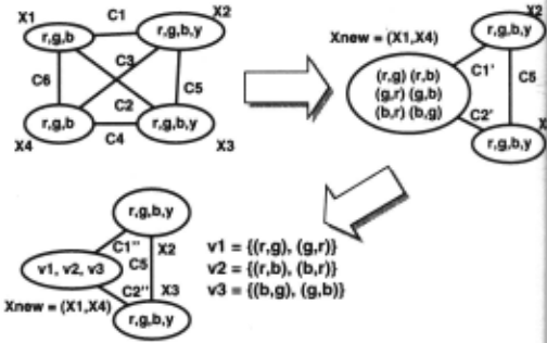
However, interchangeability is rarely valid for complete CSPs. It can often be found only for certain contexts, or for combinations of several variables. We call such combinations meta variables. The coloring example in Fig. 1 illustrates this fact. Assume that variables X1 and X 4 are clustered into a new meta variable X new. Then there are 6 values for Xnew , namely the solutions of the subproblem induced by X1 and X 4 ~ C1, C3 and C2, C4 are merged into C1' and C2' respectively. The constraint C6 will no longer appear since it is already accounted in the value combinations allowed for Xnew· The new structured value (X1 = r, X4 = g) for Xn ew is then compatible with b and y for variable X3. It turns out that by calculating interchangeability for val ues of X new, we can find three equivalence classes each of size two, namely v1 = {(r, g), (g, r)}, v2 = {(r, b), (b, r)} and v3 = {(b,g),(g,b)}. These are the meta values for X new. One solution of the transformed CSP is (X new =

v1, X2 = b, X3 = y) and this solution represents the two detailed solutions (X1 = r, X2 = b, X3 = y, X4 = g) and (X1 = g, X2 = b, X3 = y, X4 = r) . This small example shows that one can find interchangeability in problems after solving a subproblem, although no in terchangeability could be found in the original problem formulation . In [Freuder, 1991], Freuder gives an al gorithm for computing neighborhood interchangeability which runs in O(n 2 d 2 ) time, where n is the number of variables and d is the maximal domain size. This algo rithm and its extension to k-interchangeability are the only polynomial time algorithms to find all interchange able values in CSPs known so far. Finding all fully inter changeable values [Freuder, 1991) of a CSP, for example, requires finding all its solutions and is thus intractable in general. Thus we only consider neighborhood inter changeability. In order to compact the search space, we calculate neighborhood interchangeability in meta CSPs, and identify thereby meta-interchangeability as described in [Freuder, 1991]. We will first present the structuring algorithm. Then we describe an algorithm to calculate interchangeability for values of meta variables and illus trate in 4 the structuring algorithm with an example. In sec. 5 we describe a model for CSPs with clustered con straint graphs and conclude after an empirical evaluation of the algorithm.
2 The Structuring Algorithm
The various steps in the structuring algorithm are de picted in Fig. 2. A clustered structure of a constraint graph can be made explicit in the first step using graph partitioning algorithms. After having identified the clus tered structure, it can be exploited for finding inter changeability and consistency in the meta CSPs that are generated iteratively. The iteration of calculating in terchangeability and running consistency in meta CSPs continues until a single meta variable is created for each cluster identified by the graph partitioning step. Thus the amount of preprocessing that needs to be invested in the iteration depends on how many clusters the graph is decomposed .
Graph Partitioning: Given a CSP with clustered constraint graph G(V, E), we apply a graph decompo sition method called the Recursive Bisection Partition ing [ Ciarlet et a/., 1994] that allows us to identify a set of edges Ep, which, if removed, decompose the constraint graph into several connected components. For clustered graphs, one can expect that the set Ep corresponds to the intercomponent edges of the graph, and each con nected component that remains after removing Ep, cor responds to a cluster with higher connectivity. The prob lem of finding a minimum cut bisection of a graph is a well known NP-complete problem [MacGregor, 1978], and among the heuristics for finding an approximation to the problem the Recursive Bisection Method [Ciarlet et al., 1994] is a very successful one. It recursively ap plies the median cut partitioning method that could be described as follows:
- Build the Laplacian matrix of the graph G, which is basically the adjacency matrix of the graph G and in the diagonal we put -ladj(X;)I . Then calculate the second smallest eigenvalue of the matrix and the corresponding eigenvector f, which is called the fiedler vector [Fiedler, 1973].
- Let x1 be the median value of the components of the fiedler vector f. Node X; will be put in cluster C1 if its corresponding position /; is smaller than x1, otherwise node X; belongs to cluster C2.
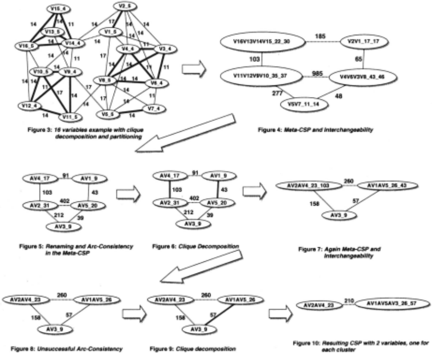
Consider the example from Fig. 3. The median cut pro cedure partitions the graph into clusters C1 = V1, ... , V8 and C2 = V9, ... , V16 indicated by hachted edges Ep. A stopping criteria for the recursive part of the algorithm needs to be defined. The recursion stops when the num ber of edges that should be removed in each step is big ger or equal to the number of edges that rest in each component. In an interactive mode, the user might be prompted and asked for the decision.
For every cluster we can identify a subset of nodes VE that are linked with nodes in other clusters, and a set of nodes VI having only internal links. The nodes VE can act like a set of articulation nodes that limit the in teraction of assignments to the nodes VI with the other clusters. At the same time, these nodes are intuitively the part of the cluster through which value interaction is transmitted among the different clusters. Thus by find ing consistent assignments to the variable in VE, we can localize the effects of assignments to the other variables of the CSP. The clustered structure is therefore a major source for interchangeability. In the example described in sec. 4, we cluster the variables V13, V14, V15, V16 into a new meta variable AV 4. Any set of values for A V 4 that have the same assignments for the variables in VE = V13, V14, V15 are interchangeable wrt. the rest of the CSP.
Meta CSPs: Variables, inducing subproblems of the CSP, are clustered together and treated as a single meta variable. Each solution to a subproblem is a composed label of the size of the subproblem and becomes a value of the new meta-variable. Adjusting the constraints must in turn be done for all the values of each new variable. Values of the new variables are compatible wrt. the new constraint if all pairs of the compound labels are com patible wrt . the original constraints. The result is called a meta CSP in [Freuder, 1992] . There are many reasons why it can be interesting to cluster variables: the result ing meta CSP might have a nice structure so that it can be solved efficiently. This is the case in the tree cluster ing procedure [Dechter and Pearl, 1989] where variables are clustered together such that the resulting meta CSP is a tree . The ultimate goal, pursued here, is to find clusters of variables such that their values are meta in terchangeable.
There are many possible subproblems that could be clustered together. The clustering procedure presented here will satisfy the following two conditions: 1) the nodes should be tightly connected because the domain size for the new variable should be kept reasonably small 1 , and 2) the nodes should belong to the same clus ter identified by the graph partitioning method. There fore we use a greedy maximal clique decomposition a~o rithm, described next, applied on the graph G(V, E\Ep) · A greedy clique decomposition algorithm of a graph G partitions the nodes of G into cliques 2 · To find such a decomposition, one starts with a single node and builds successively a bigger clique by putting nodes into the clique that are adjacent to all the nodes already in the clique until the clique cannot be extended further i.e. no other node is adjacent to all the nodes in the clique. Having found such a maximal clique one removes all the nodes in the clique from the graph. The algorithm fi nally stops when no nodes are left in G. There are many possible clique decompositions and a heuristic that al ways selects a node with the highest degree to be put into the current clique is used. An example of such a decomposition can be found in the example in Fig. 3, where the cliques are indicated with bold edges.
Using the clique decomposition as a heuristic to cluster variables can be justified by the fact that these problems are highly connected and thus might not allow many solutions that appear as new values for the meta variable in the next step. This heuristic corresponds partly to the maximum degree variable ordering heuristic [Dechter and Meiri , 1994] in backtrack search.
Interchangeability and Consistency: Calculating interchangeability for the values of the meta variables allows us to reduce the size of the CSP when sets of val ues can be treated as a single value. From the definition of neighborhood interchangeability one can see that the chance for finding these interchangeable values increases with a decreasing number of constraints that have to be checked. Thus the heuristic to choose cliques for clustering described above might result in more interchangeable sets of values compared to a random clustering.
1 The new domain size is exponential in the size of the subproblem.
2 In the literature, however, clique decompositions often partition the edges and not the nodes into cliques.
When clustered variables have been replaced by meta variables, arc-consistency might find additional inconsis tencies which were no apparent in the original problem. These pruned meta values are actually partial solutions of the original CSP that cannot be extended to a global solution.
3 Calculating Interchangeability
In this section we present another algorithm to iden tify interchangeable values for meta variables. The basic idea is to take advantage of the set of articulation nodes VE already presented in section 2. In order to identify interchangeability of two values v1 and v2 of a meta variable X with Freuder's algorithm, one needs to iter ate over all constraints that link X with its neighbors and check if exactly the same tuples are valid for v1 and v2. For two values having the same assignments for the variables in VE , we do not even have to check the con straint, because the same assignments to VE imply the same allowed tuples for the constraints. Thus these val ues are interchangeable. The following algorithm runs faster than Freuder's algorithm, but might not find all sets of interchangeable values.
Algorithm 1 Interchangeability of Meta Values Let X be a meta variable created by clustering the set of variables V (V = V1 U VE):
- Identify VE ~ V .
- Unless VE = V, iterate over the values of a meta variable X and use the projection of the compound labels of each value onto the set VE to discriminate between the different equivalence classes of inter changeable values.
One can show that the interchangeable sets for values in a meta CSP found by algorithm 1 are always sub sets of the interchangeable sets found by Freuder 's al gorithm. Thus, to find all interchangeable values, it is proposed to run algorithm 1 followed by Freuder's algo rithm. Although this results in the same interchangeable sets as when running Freuder 's algorithm only, it can be much faster . Algorithm 1 runs in O(dn) time 3 . Thus the complexity of Freuder's algorithm can be calculated by O(D 2 n 2 ) where D is the number of equivalence classes returned by algorithm 1. Most experiments done so far indicate that the sets not found by our algorithm are rare. This is not very surprising knowing that inter changeability applied directly on CSPs is also rare.
3 d, n are the domainsize and the number of variables of the metaCSP.
4 Example
Fig. 3 shows the constraint graph of a CSP with 16 variables. Every variable name is followed by its domain size and every constraint is labeled with the number of tuples allowed by the constraint. The me dian cut partitioning finds 4 edges between the nodes (V14, V2),(V14, V1),(V9, V5) and (Vll V8) that parti tion the graph into cluster V1, V2, ... , V8 and a sec ond cluster V9, V10, .. . , V16. The partitioning algo rithm is then stopped and the iteration on building the meta CSP calculating interchangeability and run ning consistency is repeated until a single meta variable is created for each cluster. The greedy clique decom position algorithm determines in the first run 5 sub problems with complete graphs indicated by the bold edges in Fig. 3. Every subproblem is solved individ ually and appears in Fig. 4 as a new meta variable. The variables V13, V14, V15 and V16 for example are clustered together into the meta ·variable, named "V16V13V14V15". The number of solutions of this sub problem is 30, i.e. the last number of the node label. Interchangeability identifies 8 equivalence classes of values each of size 2. Thus the domain size can be reduced to 22. As an example of a set of interchangeable values consider S1 = (V16 = 0, V13 = 4, V14 = 2, V15 = 3) and S2 = (V16 = 0, V13 = 4, V14 = 2, V15 = 2) . One can see how the nodes V16, V13 and V14 act as the articulation nodes VE. Algorithm 1 finds the set VE, the projection of S1 and S2 onto VE is (V16 = 0, V13 = 4, V14 = 2) for both values, and thus S1 and S2 are interchangeable. Renaming V16V13V14V15 to AV4 (AV stands for Abstract Variable) and applying arc-consistency to the CSP is shown in Fig. 5. With arc-consistency one can remove 5 values from the domain of AV 4. The four edges found by the graph partition ing in the first step corresponds now to the three edges (AV1, AV4),(AV2, AV5) ,(AV2 , AV3) that are not al lowed to appear in a clique in the next step. Conse quently two new clusters AV1AV5 and AV2AV4 are created and AV3 is not changed (Fig. 8). In a third step "AV1AV5" and AV3 are clustered together resulting fi nally in a CSP with two nodes AV2A V 4 with domain size 23 and AV1AV5AV3 with domain size 26. These two nodes corresponds to the two clusters V1, V2, ... , V8
and V9, V10, ... , V16 determined in the first step. 210 tuples are allowed by the constraint between the two nodes and these tuples correspond to the solutions for the CSP on this level (Fig. 10). Every meta-value in a solution of the resulting CSP can be replaced by the set of values it represents. In this way one obtains the cross product representation [Hub be and Freuder, 1992] of so lutions for the next lower level. Replacing meta values for each solution in the crossproduct continues until the lowest level is reached. The 210 solutions can be refined to 43B on the next lower level then to 2910 and finally to the 5366 solutions of the original CSP. It is worth to mention that the size of the equivalence classes of values plays a multiplicative role when determining the number of solutions on the next lower level. If a solution S con tains t meta values that represent classes of size s; with i = 0, .. . , t- 1, then the number of solutions on the next level that are represented by s equals n::~ s;.
5 Clustered Constraint Graphs
Constraint graphs of problems that arise for exam ple from physical interactions often resemble clustered graphs. We shortly describe a simplified model for gen erating clustered graphs, however details can be found in [Hogg, 1996]. The nodes of the graph to be gener ated will appear as the leaves of a balanced binary tree. Thus to generate graphs with 2D number of nodes we build a balanced tree with depth d = D - 1. The 'tree induces a ultrametric distance between pairs of nodes, defined as the number of levels up in the tree from the nodes to reach a common ancestor. For a given p with 0 < p < 1, edges in the graph between nodes at distance t (0 < t ~ d) can then be selected with a relative probabil ity p 1 . As an example consider the clustered constraint graph in Fig. 3. The nodes V1, .. . , V16 are the leaves of a balanced tree with depth 3 arranged from left to right in increasing order. Given p = 0.5 the probability of having an edge in between two nodes from the set V1, ... ,VB and from the set V9, ... , V16 is 0.5 3 = 0.125. An edge in be tween two nodes in V1, ., V4 and V5 .. , VB appears with probability 0.25 etc. . Having build the clustered graph one can easily construct a CSP with clustered constraint graph by randomly selecting domain sizes and allowed tuples for the constraints.
6 Evaluation
Any evaluation of a technique depends on the ob jectives it is used for . Our objective is to struc ture a CSP so that its solution space can be eas ily inspected. Thus, a reasonable measure would be the average number of choices a user has to make to select one particular solution among all possibili ties. The results for a small number of test cases generated with n = 32 , p = 0.4, domainsize = 3, I Testcase 4: ;fter 1 iteration IOQ(34602) = 10.45
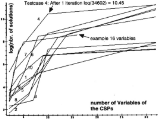
number of constraints = 110 , 70% from all possible tu ples for each constraint are allowed , can be found in Ta ble: 1 and in Fig. 11 . The problems are tranformed until CSP with two variables are returned. Over-constrained problems and problems with Jess that 100 solutions are omitted. We define a condensing factor of the solu tion space p; = logisolutions level; lflogiall solutions! with 1/logiall solutions! ~ p; ~ 1 and for different abstraction levels i = 0, . .. , k. Using this measure, we can discriminate between CSPs where the algorithm returns good and bad results 4 . A factor close to 0 implies a very condensed representation, while a fac tor of 1 could not condense the solution space much. A series of runs confirm the intuition that for clus tered CSPs with "many" solutions, the number of so lutions of the resulting meta-CSPs is condensed con siderably, often by a large factor (see. Fig. 11). Test case 2 for example could be condensed from 2066 so lutions to 6 solutions after 3 iterations. Resulting in a P3 = log6jlog2066 = 1.7917595/7.6333694 = 0.234. Thus, the structured problem will considerably reduce the effort required to search through the solution space of such a CSP.
The evaluation method needs to enumerate all solu tions for the condensed CSP. This, however, is only pos sible for small CSPs. For large CSPs (i.e. when the re sulting CSP has still> 100 variables), we will use a prob abilistic approach that determines the expected number of solutions of the CSPs (based on [Knuth, 1975]) on the different levels to determine p;.
4 pis not defined for CSPs with only a single solution
| Solutions on level : | Example and Testcases 1 - 10 | ||||||||||
|---|---|---|---|---|---|---|---|---|---|---|---|
| Ex.(16 vars) | 1 | 2 | 3 | 4 | 5 | 6 | 7 | 8 | 9 | 10 | |
| 3 | 210 | 36 | 6 | 11 | 26 | 22 | 15 | 15 | 9 | 24 | 43 |
| 2 | 438 | 84 | 26 | 17 | 1428 | 76 | 184 | 235 | 30 | 180 | 146 |
| 1 | 2910 | 188 | 862 | 1550 | 34602 | 4260 | 4832 | 6220 | 951 | 5712 | 904 |
| original CSP | 5366 | 2632 | 2066 | 2750 | 74718 | 54280 | 25872 | 77828 | 1512 | 48972 | 1460 |
| P3 | o.62 | 1 0.44 | 1 o.23 | 1 o.29 1 | o.28 | 1 o.21 | 1 o.26 | 1 o.23 | 1 o.28 1 | o.28 | 1 o.5o |
7 Future Work and Conclusion
In this paper we have presented a structuring method for CSPs. Applying the method to a CSP results in a more condensed representation that allows the enumeration of sets of similar solutions and thus facilitates the selection of single solutions. One should contrast this with search algorithms for solutions in the original CSP: They find one solution after the other without showing the similar ity in between them. Furthermore, in many applications it is not enough to present a human decision maker with a single solution, because this single solution might vio lates other criteria which the user has not made explicit to the problem. Thus one should give the user a chance to integrate hidden knowledge and unquantifiable prefer ences in the decision process by proposing sets of similar solutions from which he can make the selection.
The evaluation of our algorithm imposes many diffi culties and a lot of work needs still to be done. It is for example not enough to know how many interchangeable sets we get and how big they are; it is very important to know in how many solutions a meta value will finally appear. This always requires us to look at all solutions of a CSP, a set which is impossible to generate for large CSP. In the future work we will also look at hard ran dom problems. Basically one would like to compact the search space such that certain instantiations might have to be made only once for each equivalence class of val ues, thus reducing the search effort. Similarly these hard problems often exhibit a high degree of consistency and thus low consistency algorithms will not find inconsisten cies. Running arc-consistency on a meta CSP, which is related to restricted form of k-consistency with k equal to the sum of size of two adjacent clusters, might therefore be very interesting for hard CSPs.
@inproceedings{ijcai1997p62,
  title     = {Structuring Techniques for Constraint Satisfaction Problems},
  author    = {Weigel, Rainer and Faltings, Boi},
  booktitle = {Proceedings of the Fifteenth International Joint Conference on
               Artificial Intelligence, {IJCAI-97}},
  publisher = {International Joint Conferences on Artificial Intelligence},
  editor    = {Martha E. Pollack},
  pages     = {418--422},
  year      = {1997},
  note      = {Constraint Satisfaction},
  url       = {https://ijcai.org/proceedings/1997/62},
}
TY - CPAPER TI - Structuring Techniques for Constraint Satisfaction Problems AU - Weigel, Rainer AU - Faltings, Boi T2 - Proceedings of the Fifteenth International Joint Conference on Artificial Intelligence, IJCAI-97 PB - International Joint Conferences on Artificial Intelligence PY - 1997 SP - 418 EP - 422 UR - https://ijcai.org/proceedings/1997/62 ER -Copied
Machine-readable versions of this paper, for tools and AI agents:





