
Local Consistency for Ternary Numeric Constraints
Proceedings of the Fifteenth International Joint Conference on Artificial Intelligence. Constraint Satisfaction. Pages 392-396.
© 1997 International Joint Conferences on Artificial Intelligence
Abstract
We consider algorithms of the Waltz type for computing local consistency (also called arcconsistency) for constraints over numeric domains. Many commonly used propagation rules do not in fact enforce local consistency. We extend the propa&ation rule given by Faltings [Faltings, 1994j to the case of ternary constraints. Since any general n-ary continuous constraint can be represented as a collection of ternary ones, this also covers n-ary constraints in general. We show how the propagation can be implemented efficiently. The new algorithm gives significantly tighter labellings than previous propagation algorithms on most problems.
- -10, 10) l-10, 10J l-10, 101 x2 [-10, 7.2] [-10,10] [-8, 85, 7.2] x3 [-10, 10] [-10,10] [-10,10] x~ [-10, 5.25] [-10, 5.25] [-10, 5.25] x6 [-6.86, 7.33] [-10, 7.33] [ -5.35, 7.33] Xe [-10, 10] [-10,10] [-9 .84, 10] x1 [-9.4, 10] [-10,10] [-9.4, 10] Xs [-10, 9.4] [-10, 10] [-10, 7.16] Xs [-4.6, 10] [-4.6, 10] [-3.41, 10] X1o [-10, 10] [-10, 10] [-10,10]
- [Benhamou et al., 1994] F. Benhamou, D. McAllester, P. Van Henten- ryck: "CLP(Intervals) Revisited," Technical Report No. CS-94-18, Universite Aix-Marseille, April 1994
- [Davis, 1987] Ernest Davis: "Constraint Propagation with Interval Labels," Artificial Intelligence 32, 1987, pp. 281-331
- [Faltings, 1994] Boi Faltings: "Arc-consistency for continous variables," Artificial Intelligence 65, 1994, pp. 363-376
- [Freuder, 1982] Eugene Freuder: "A sufficient condi- tion for backtrack-free search," Journal of the ACM 29(1), 1982, pp. 24-32
- [Hyvonen, 1992] E. Hyvonen: "Constraint reasoning based on interval arithmetic: the tolerance propaga- tion approach," Artificial Intelligence 58(1992), pp. 71-112 [
- [Lhomme, 1993] Lhomme: "Consistency Tech- niques for Numeric CSPs," Proceedings of the 13th IJCAI, 1993, pp. 232-238 IJCAI
- [Sam-Haroud and Faltings, 1996] Djamila Sam- Haroud, Boi Faltings: "Consistency Techniques for Continous Constraints," Constraints 1(1), 1996, pp. 85-118
- [Waltz, 1975] David Waltz: "Understanding line drawings • of scenes with shadows," in P.H. Win- ston( ed. ): The Psychology of Computer Vision, McGraw-Hill, NY 1975
References were extracted automatically from the PDF and may contain errors.
Full text extracted automatically from the PDF; figures, tables and equations may differ. The PDF is the version of record.
1 Introduction
The constraint satisfaction problem (CSP) is ubiquitous in many practical applications. We consider in particular CSPs with continuous-valued variables, given by:
- a set of variables {Xi}·
- a set of ternary constraints Cx,,xi,x,., defined as inequalities f(xi, Xj, xk) ;::: 0. Note that an equal ity f = 0 can be modelled as a conjunction of two inequalities f;::: 0 and f ~ 0. Binary and unary con straints are defined similarly with the corresponding number of variables.
A solution to a CSP consists of value assignments {Xi = xi} to all variables such that all constraints are satisfied. Throughout this paper, we use upper case letters for variables and lower case letters for particular values.
For linear constraints, there are efficient optimization algorithms for finding single solutions to CSPs. For non linear constraints, optimization algorithms only apply to special cases. More importantly, there are many appli cations in configuration, diagnosis or planning where it is important to know not a single solution, but the space of all possible solutions. Algorithms for determining the space of all solutions also find applications in numeri cal analysis ([Benhamou et al., 1994]). A solution space can be represented by a set of labels defining the consis tent values or value combinations. In numeric domains, it is very difficult to represent sets of. value combina tions. However, sets of values for individual variables can be represented efficiently by collections of intervals. We consider algorithms for computing labellings which are locally consistent according to the following defini tion:
Definition 1 A labelling is locally consistent if for ev ery Xi, X; and every value Xi E Li 1 there exists a value x; E L; such that for every constraint Cx,xix,. involv irrg xi and X; and possibly another variable X k I there exists a value Xk E Dk such that Cx,,Xj,X,. is satisfied for xi= Xi,Xj = x;,Xk = Xk:
Note that this definition is different from others (e.g., [Davis, 1987]) in that it requires that one single value x; can satisfy all constraints. This ensures that the locally consistent labelling of the ternary system is at least as tight as the locally consistent labelling of its binary projection. Note that our work distinguishes itself from others, for example [Hyvonen, 1992] or [Lhomme, 1993], in that we are only considering efficient and gen eral algorithms for local consistency, without any at tempt to impose global consistency.
2 Local consistency with numeric constraints
A locally consistent labelling can be computed using the Waltz algorithm. It consists of applying a propagation rule to the labels of every variable pair until it results in no more change. While local consistency is very of ten applied for CSP with discrete domains, in continu ous domains Davis ([Davis, 1987]) has reported a num ber of very negative results, including the fact that the Waltz algorithm does not guarantee a locally consistent labelling and may often fail to terminate. [Faltings, 1994] has shown that many of his negative results are due only to an overly straightforward formulation of the propaga tion rule used in the Waltz algorithm:
- Davis assumes that only interval boundaries are propagated, but with nonlinear constraints local ex trema and intersections between constraints may also become interval bounds.
- Davis assumes that each constraint between the same set of variables is propagated individually, thus creating implicit cycles in the constraint network when several constraints involve the same variables.
The shortcomings introduced by these assumptions are already apparent in the following simple example of a parabola and a sphere:
with initial intervals of xi i = 1, 2, 3, 4 of [-10, 10] . Here, Davis' propagation rule results in no refinement whatsoever of the initial labels. · However, upon closer consideration, we find that:
- X3 can never become greater than 5. This bound is not found since it is reached at a local extremum of a constraint.
- X 3 can never become smaller than -3.36. This bound is not found since it is given by the inter section of the two constraints.
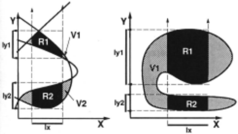
A more powerful propagation rule can be obtained by generalizing the propagation rules used in discrete do mains to the infinite, continous case. To do this, it is necessary to consider all constraints involving the same pair of variables X and Y simultaneously rather than in dividually; we call their conjunction the total constraint between X and Y . It may consist of several regions V1, .. , v.~. of feasible value combinations (Figure 1).
In a propagation step from X to Y, the label of Y is modified to exclude those values which are not com patible with any value in the label of X. This can be accomplished by first restricting the feasible regions of the total constraint to those within the label of X, called the restricted regions (Figure 1) R1, ... , Rr. Projecting these restricted regions onto the Y -axis gives the inter vals of Y -values admitted by the propagation. [Faltings, 1994] shows that this propagation rule guarantees a lo cally consistent labelling upon termination.
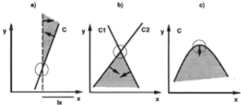
Implementing such a rule poses some difficulties, since the regions making up the totat constraint can become quite complex (see Figure 1). [Faltings, 1994] gives a method for propagation without explicitly considering the regions formed by the constraints. It is based on propagating eztrema of boundaries of restricted regions. There are three types of extrema (see Figure 2):
- intersections between constraints and interval bounds
- constraint intersections
- local extrema of constraint curves
We consider the propagation of the label of X to that of Y through a restricted region of a constraint be tween X and Y. We let B(R) be the continous bound ary of a restricted region R. Extrema are then the lo cal maxima and minima in Y of B(R) with respect to X. Note in particular that extrema here refer to the boundary B(R), not the region R itself. As a nota tion, we let ma:z:y(B(R), Yo) be true if and only if B(R) has a local maximum in Y with Y-coordinate Yo, and miny(B(R), y0 ) if it has a local minimum. Note that if R is bounded by a set of constraint curves, the extrema of its boundary B(R) are a subset of the extrema and intersections of these curves. Only those which satisfy all other constraints bounding R are valid, the others are ignored. Thus, the set of extrema can be found by purely local considerations.
We now define the function oy(R, y) to be the differ ence in the number of maxima and the number of minima at y-coordinates greater than or equal to y:
It is then possible to prove ([Faltings, 1994]) that:
- if there is a point (:z:*,y*) E R, oy(R,y*) > 0, (Lemma 2.9) and
- if there is no point (:c*, y*) E R, ay(R, y*) = 0 (Lemma 2.7)
The propagation rule should eliminate a value y* from the label Ly if and only if it is in no region, i.e. ay(R.;, y*) = 0 for all E.;. Since ay(R.;, ... ) ~ 0 for any E.;, this can be conveniently expressed as Li ay(R.;, y*) = 0. By rewriting this as:
we only require the total number of extrema in all regions taken together, without any consideration of the regions they belong to. The set of illegal y*, and conversely the set of legal y, can thus be characterized without knowing which extrema belong to which region!
The following propagation rule computes the maximal intervals of admissible y and thus achieves local consis tency (for the proof, see [Faltings, 1994]):
- compute the set MAX of local maxima and the set MIN of local minima of all restricted regions r E R(Q, I.,), Q E ct(:c, y).
- Filter both MAX and MIN to keep only those ex trema which satisfy all other constraints, i.e. ac tually bound a legal region. Order the two sets of points according to their y-coordinate (these sets are obtained directly by consideration of individual constraints c(:z:, y)).
- set inde:c <- 0, consider the extrema e in MIN and MAX in decreasing order of their y-coordinate, where elements of MAX are always considered be fore elements of MIN, and do:
- (a) if e E MAX, inde:c <- inde:c + 1. If e E MIN, inde:c <- inde:c - 1.
- (b) if inde:c has just changed from 0 to 1, set Ylow·~ <- y- coordinate( e).
- (c) if inde:c has just changed from 1 to 0, set Yupp·~ <- y-coordinate(e) and add the interval [Ylow·~ ··Yupp·~] to Iy.
5. return Iy.
We assume that all local extrema of constraints as well as constraint intersections have been precomputed be fore running the propagation, so that the computation of MAX and MIN in step 2 only requires evaluating the constraints at interval bounds; the amount of con straint mainpulation required in each propagation step is exactly the same as that of other more straightforward propagation rules based only on interval bounds.
3 Generalization to ternary constraints
In practice, constraint networks are almost never binary. The main novel contribution of this paper is to general ize the propagation rule of [Faltings, 1994] to ternary constraints over continous variables. The generalization again makes use of the property that the propagation rule only needs to know the complete set of extrema of all feasible regions, but not what regions there are.
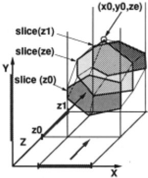
Propagation with a single third variable Z We first consider the case of propagating the label of X to Y through a set of constraints Cxyz involving a single third variable Z (see Figure 3). The consistency condi tion of Definition 1 for the label of Y is now:
We define the projection of the ternary constraint:
so that the local consistency condition for Ly for the ternary constraint Cxyz becomes the consistency condi tion for the binary constraint Pxy(Cxyz). Thus, prop agation through the projection will give a consistent la belling.
In order to apply the propagation rule, we need to de termine the extrema in the boundaries of this projection. The following lemma indicates where to find them:
Lemma 1 Assume that (:c., y.) is an eztremum of Pxy(Cxyz). Then, there must ezi8t .a z. E Lz such that (:c., y., z.) is an eztremum of Cxyz restricted to values of Z within its label Lz.
Proof:
Since (:c., y.) is in Pxy(Cxyz), there must be a z. such that (:c., y., z.) is in Cxyz. On the other hand, since (:e., y.) is an extremum in y of Pxy(Cxyz), there is a small interval of :c' around :c. such that there is no point (:c., y') E Pxy(Cxyz) withy'> y. (maximum) or y' < y. (minimum). But this means that there is no z' such that { :c', y', z') E Cxy z, which is just the condition for (:c., y., z.) to be an extremum of the ternary constraint. QED.
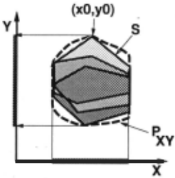
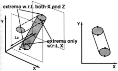
Extrema of ternary constraints can fall on interval bounds, local extrema, constraint intersections, but also combinations thereof. For example, the intersection of two constraints involving the same variables forms a curve which can have an extremum, or a constraint curve can have a local extremum in one coordinate and reach interval bound in the other. Let Z = {ze~, Ze:l, ... , Zel:} be the set of Z-coordinates of all extrema. Each Zei defines a "cut" through the space spanned by all constraints in volving X andY, called a 1lice (Figure 3). Now consider the set S:
which is the union of all slices at extrema of Z (Figure 4). The set S does not necessarily cover Pxy(Cxyz), but because of Lemma 1 it contains all extrema. However, it is not true that the union of all extrema of slices in S will give the correct propagation, since it also contains interior extrema which would lead to false gaps during propagation. For example, the propagation shown in Figure 5 generates disjoint slices even though the projection should be one continous region.
These interior extrema are characterized by the fact that they are not also extrema of Cxyz with respect to Z. Thus, the set of extrema E of Pxy ( C XY z) is the set of all extrema of some slice which are also extrema with respect to Z. We can show the following:
Lemma 2 Updating the label of Y by propagating Lx through E will give the 1ame re1ult a6 propagating it through Pxy(Cxyz), and thu1 through Cxyz it1elf.
Proof:
Interval bounds of Py(Cxyz) can only fall on extrema of Pxy(Cxyz) and thus of Cxyz itself. By construction, E contains all extrema in Y of Pxy(Cxyz), with the interior ones filtered out. Thus, the projection of S onto the Y -axis will be identical to that of Pxy ( C XY z). QED
and we have a correct propagation rule for a set of constraints with a single third variable.
Propagating constraints with several third variables When there are several third variables Z1, Z:l, ... , Zl: with constraints Cxyz,, labels must be propagated through their inter1ection. Since the third variables are all distinct, the projection of their intersec tion is the intersection of the projections, i.e.:
This intersection can be carried out implicitly by (i) fil tering all extrema (:z:., Ye) such that for some third vari able z,, there does not exist a Zei such that (:z:e, Ye, Zei) satisfies Cxy z,, and (ii) adding all extrema resulting from intersections of Cxyz, and Cxyz;-
Identifying slices Slices need to identify all points which could possibly give rise to extrema of the pro jection Px,x; of a constraint. Consider thus a total constraint Ck.x; = {C}.x;z 1 , ··· ,ctx;z,J involving k other variables zl··zl:.
The first set of slices to be considered are those which fall at interval bound1 of some z,. The second set of slices to be considered are local extrema of individual constraint curves. Consider a single ternary constraint CxYZ;.· It has a local extremum in Y at (:z:e, Ye, ze) if both:
- either 6Cj6X(:z:e, Ye, Ze) bound 0 or :Z:e 1s an interval
- either 6C /6Z(:z:e, Ye, ze) = 0 or Ze is an interval bound
The set of relevant slices is obtained by considering all constraints which involve X and Y and collecting all Ze satisfying the above conditions and falling into the label of z,, Lz,.
The third set of slices is generated by inter1ection6 between constraints. Here, the situation can be quite The is the case exactly if the normal vectors of both con straints lie in a plane that also includes the Y -axis, i.e. n( (\) + an( C2) is a vector parallel to the Y axis, for some a. This leads to a system of equations for such extrema which can be solved using numerical methods.
The binary propagation rule is thus adapted to ternary constraints by replacing step 2) as follows:
- add to MAX all local maxima and to MIN all local minima of all restricted regions B. in the slice ct(:z:, y, z.,), obtained directly by con sideration of individual inequalities and their intersections.
- filter from MAX and MIN all those extrema which are not also extrema with respect to z,.
- for all other constraints Cxy z~, Z1e E Z filter from MAX and MIN all those extrema which are not satisfiable by the constraint Cxy z~, and add all extrema which correspond to in tersections between a constraint C XY z, and Cxyz~·
The following theorem shows that using this propa gation rule in the Waltz algorithm results in a locally consistent labelling:
Theorem 1 The ternary propagation rule reache6 qui e6cence only when the label6 are locally con6i6tent.
Proof:
Follows from the correctness of the binary propagation rule (Theorem 2.1 in [Faltings, 1994]) and the equiva lence of propagating through S and Pxy. QED
Example of a propagation step. We consider the propagation of X1 to X 3 in the system of constraints already mentioned in section 2:
with four variables xl, .. , x4 and initial labels of [-10, 10] for X1 to X4 . The total constraint is thus formed by {G1 , G2}. G2 has a maximum in Xa at {X1 = 0, Xa = 5, X4 = 0} and a minimum in X 3 at {X1 = 0, Xa = -5, X4 = 0}. The projections on X 2 and X4 of combinations of extrema (individual extrema and interval bounds) in X a give rise to the following potential slices:
For each of the slices defined by substituting combi nations of these values in the constraints, the label of XI. [-10, 10], is propagated to X3 · Only the slices (X2, X4) = (-10, 0) and (10, 0) give rise to valid extrema
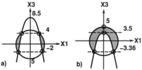
(i.e. satisfying all other constraints); they are shown in Figure 6. The result propagating X1 to X 3 through the total constraint formed by G1 and G2 is then obtained by collecting the valid extrema produced by these slices. The first slice with (X2 , X4 ) = ( -10, 0) has two MAX IMA in Xa at {X1 = ~3, Xa = 4} and {X1 = 3, Xa = 4} and two MINIMA in Xa at {X1 = -4.583, Xa = -2} and {X1 = 4.583, X 3 = -2} all of them resulting from intersections. The second slice (X2, X4) = (10, 0) has two local MAXIMA at {X1 = 0, X 3 = 3.5} and {X1 = 0, X3 = 5} as well as two MINIMA produced by intersections at {X1 = -3.7, Xa = -3.359} and {X1 = 3.7, Xa = -3.359}. Ordering all extrema in X3 and applying step 4 of the propagation rule gives the single consistent interval [-3.359, 5). In this example, the Davis method does not alter the labels ([-10 .. 10] for all variables) at all, whereas our propagation rule gives X 1 = [-5, 5], X 2 = [-10, 10], X 3 = [-3.359, 5) and x4 = [-5, 5].
4 Performance on random examples
In this section, we would like to compare our algorithm with the propagation of individual constraints ([Davis, 1987]) and show on randomly generated examples why our algorithm is better than Davis'. Numeric values in these examples are all rounded on 2 decimals.
Supposing that the restricted region always falls within the propagated intervals, we applied Davis prop agation to the following examples:
Constraint set 1
C1 -4 *X& - Xe + 6 *X; + 6 > 0
C2 4 * X, - 9 *X& - 5 * X a - 5 > 0
c3 -9 * X2 + 1 * x3 + 4 * x5 + 4 > o
C& X, + X1 - Xa - 1 > 0
C, -Xe + 10 *X; - 4 * X1o - 4 > 0
Ce -4 *X,+ X1- Xa + 1 > 0
C1 -6 * X3 - 2 *X& + 6 * Xe + 6 > 0
Ca 6 * X2 - X, + 7 *X& + 7 > 0
c; 8 * x1 - 5 * x2 - 8 * x3 - 8 > o
| X; | Local C. | Davis | Simplex |
|---|---|---|---|
| x1 x2 x3 x~ x6 Xe x1 Xs Xs X1o | II [-10, 10) [-10, 7.2] [-10, 10] [-10, 5.25] [-6.86, 7.33] [-10, 10] [-9.4, 10] [-10, 9.4] [-4.6, 10] [-10, 10] | l-10, 10J [-10,10] [-10,10] [-10, 5.25] [-10, 7.33] [-10,10] [-10,10] [-10, 10] [-4.6, 10] [-10, 10] | l-10, 101 [-8, 85, 7.2] [-10,10] [-10, 5.25] [ -5.35, 7.33] [-9.84, 10] [-9.4, 10] [-10, 7.16] [-3.41, 10] [-10,10] |
Constraint set 2
- -16 + ..L * Xg * X6 +!. * Xe-! * X6-! * Xs13 10 13 6 I 6 ~·L·h- 60 ·h·h+~·h·h+ 6 * x6 * x6 + ~ * x9 * x9 < o
- 4 * x~ - 9 * X6 - 5 * Xs - 5 > o
- -9 * x2 + 1 * x3 + 4 * x6 + 4 > o
- _! * X1o-! * Xe +.!.. * X1o * Xg +.!.. * Xe * Xg+ 1 6 6 17 10 1 10 1 lO * Xe * X1o + ~ * Xs + 6o * Xg * Xs + "i * Xe * Xe+ "i * X1o * X1o - 3 < 0
- -6 * X3 - 2 * X6 + 6 * Xe + 6 > 0
- 6 * x2 - x~ + 1 * x6 + 1 > o
- 8 * x1 - 5 * x2 - 8 * x3 - 8 > o
A comparison of the results of Davis' algorithm and the local consistency rule (Table 1) reveals that local consistency prunes labels more drastically as it consid ers intersections between constraints defined on the same pairs of variables. X5 is an example of such a variable in volved in several constraints. When compared with the simplex algorithm, which computes the globally optimal solution for constraint set 1, the labels of X2 , X5 , X1 and X8 show that local consistency is better than the Davis rule although it does not achieve global consistency. In the second example, two nonlinear constraints C1 and C4 have been added to a set of linear inequalities. Here, the local consistency algorithm is far better because, ad ditionally to label boundaries, it takes into account the individual extrema of nonlinear constraints (Table 2).
We randomly generated about 300 mixed constraints sets similar to constraint set 2. For each solution we evaluated the average number of labels different from the initial label and how much the labels had been reduced on average. Davis' algorithm reduced 3 out of 10 labels whereas local consistency reduced nearly 7 labels. The amount of pruning was 7.48% for Davis and 25.97% for local consistency.
5 Conclusions
Among all techniques developed for constraint-based reasoning, local consistency and its weaker variants such as forward checking are by far the most widely used tech niques in practice. This is due to the fact that it can be computed efficiently but still provides dramatic pruning of the search space, especially when some variables are already assigned values.
| X; | Local Consistency | Davis , |
|---|---|---|
| x1 x2 x3 x~ x6 Xe Xs x9 X1o | l-10, 10J [-10, 7.15] [-10, 5.32] [-10,10] [-4.6, 7.16] [-4.37, 2.79] [-10, 10] [-6.35, 4.24] [-6.91, 10] | l-10, 10J [-10, 10] [-10, 10] [-10, 10] [-10, 9.44] [-10, 10] [-10, 10] [-10, 10] [-10, 10] |
In continuous domains, straightforward implementa tions of Waltz pro:pagation does not guarantee useful re sults {[Davis, 1987J). A modified propagation rule which guarantees local consistency has been given in [Faltings, 1994] for binary constraints. In this paper, we have shown how the rule can be generalized to ternary and thus n-ary constraints. The Waltz algorithm using the new propagation rule gives significantly better results than the commonly used propagation rule analyzed by Davis. This result should allow significant improvements in many applications of local consistency.
@inproceedings{ijcai1997p58,
  title     = {Local Consistency for Ternary Numeric Constraints},
  author    = {Faltings, Boi and Gelle, Esther M.},
  booktitle = {Proceedings of the Fifteenth International Joint Conference on
               Artificial Intelligence, {IJCAI-97}},
  publisher = {International Joint Conferences on Artificial Intelligence},
  editor    = {Martha E. Pollack},
  pages     = {392--396},
  year      = {1997},
  note      = {Constraint Satisfaction},
  url       = {https://ijcai.org/proceedings/1997/58},
}
TY - CPAPER TI - Local Consistency for Ternary Numeric Constraints AU - Faltings, Boi AU - Gelle, Esther M. T2 - Proceedings of the Fifteenth International Joint Conference on Artificial Intelligence, IJCAI-97 PB - International Joint Conferences on Artificial Intelligence PY - 1997 SP - 392 EP - 396 UR - https://ijcai.org/proceedings/1997/58 ER -Copied
Machine-readable versions of this paper, for tools and AI agents:





