Comparing Random Starts Local Search with Key Feature Matching

1 Introduction

To find an object, recognition algorithms often first seek small sets of features which predict the object's presence. This ideas is articulated by Roberts [Roberts, 1965] and is the heart of lo­ cal feature focus [Bolles and Cain, 1982]. It suggests the value of perceptual organization [Lowe, 1985] and is fundamental to the alignment approach [Huttenlocher and Ullman, 1990]. It is also a basic component of Geometric Hashing [Lamdan et al., 1990] and continues to be refined [Olson, 1995].

Here we present a variant upon this general theme which searches for an optimal match by first searching for good matches between triples of object model and image features. For simplicity, we call this our key feature algorithm since the search for a good triple may be thought of as a searc~ for a key feature which determines the rest of the match. The key feature algorithm uses the same criterion function as our lo­ cal search line matching algorithms [Beveridge et al. , 1990; Beveridge, 1993; Beveridge et al., 1997] and this enables us to report on a set of side-by-side comparisons between the two. Since these two algorithms search the space of possi­ ble matches in very different ways, the comparison highlights strengths and weaknesses of each.

"This work was sponsored by the Defense Advanced Research Projects Agency (DARPA) Image Understanding Program under grants DAAH04-93-G-422 and DAAH04-95-J-0447, monitored by the U. S. Army Research Office, and the National Science Founda­ tion under grants CDA-9422007 and IRI-9503366

The greatest difference between the two algorithms is in how they initiate search. The key feature algorithm initiates indepdent searches from each of a set of ranked key features. Local search starts a number of independent trials from ran­ domly selected matches. The key feature algorithm relies on one or more of the key features belonging to the best match. In contrast, local search makes no effort to find consistent initial matches and instead relies upon iterative improvement guided by updated global alignment to move search from the random match to one which is good. Randomness is important to local search because the probability of failing to find a good solu­ tion over multiple trials drops exponentially as the number of trials increases. This same random sampling methodology has been used in the RANSAC algorithm to find consistent sub­ sets of object model and image features [Fischler and Bolles, 1987].

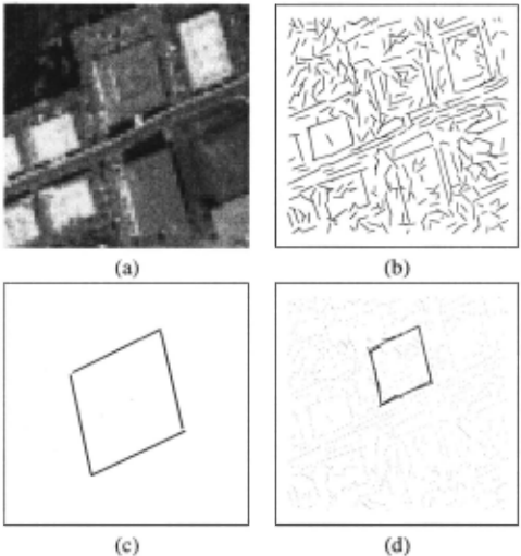
We begin by reviewing our formulation of2D line segment matching as a combinatorial optimization task which has as its goal finding matches such as the one shown in Figure I . Next the random-starts local search and key feature algorithms are described and their performance is compared on the example just shown as well as on a series of controlled test problems.

2 Optimal Matching

Let M be a model of 2D line segments and D a set of seg­ ments representing image data. A match is a many-to-many correspondence mapping c where:

An objective function E defines the best match c*.

The match errorE has two terms [Beveridge, 1993]:

Efit(c) measures how well the model fits the data. Eom(c) measures how much of the model is omitted from the match.

To evaluate E, a 2D similarity transformation best fitting the model to the data is computed. The fitting criterion is a weighted sum of integrated perpendicular distance between infinitely extended model lines and their corresponding data line segments: ERes (c) is a normalized function of the resid­ ual error after fitting. The best fit for any c, neglecting under­ constrained cases, is computed by solving a quadratic polyno­ mial. Eom (c) is computed by transforming the model to the best-fit configuration and measuring how well the data covers the model. The weighting term <J dictates how far a data seg­ ment can be from a model segment and still be included in an optimal match. If, for instance, <J = 3, then the data may be up to 3 pixels from the model.

3 Random Starts Local Search

Perhaps the simplest algorithm is steepest-descent on a 'Hamming-distance-I' neighborhood. This is so named be­ cause any correspondence mapping c may be represented by a bitstring of length n, where n E IS 1. A 'I' in position j of the bitstring indicates that the jth pair in the set S is part of the match c. The n neighbors of c are generated by succes­ sively toggling each bit. Hence, the neighborhood contains all matches created by either I) adding a single pair of model-data features not already in the match or 2) removing a single pair currently in the match.

Steepest-descent local search using this neighborhood com­ putes E for all n neighbors of the current match c, and moves to the neighbor yielding the greatest improvement: the great­ est drop in E. Search terminates at a local optimum when no neighbor is better than the current match.

Because local search often becomes stuck at undesirable lo­ cal optima, it is common practice to run multiple trials. Each trial is started from a randomly chosen initial match c;. The random selection of c; is biased to choose, on average, A data segments for each model segment. Specifically, let hm be the number of pairs in S which contain a model segment m. Each of these pairs is included in c; with independent probability *. Our experience suggests A = 4 is a good choice, thus binding on average 4 data segments to each model segment.

Over t trials, the probability of failing to find a good match drops as an exponential function oft. Let P 8 be the probability of finding a good solution on a single trial. The probability of failing to find a good match in t trials is:

For geometric models, there is often a well defined and known best solution and we can characterize algorithm performance in terms of the probability P8 of finding the best match in a given trial. From P8 , the required number of trials t8 needed to solve a particular problem to a preset level of confidence Q8 may be derived from equation 5:

4 Key Feature Matching

The local search algorithm just presented can be turned into a key feature matching algorithm by initializing search from k carefully selected key feature matches. Let F be the set of key features, and let a specific key feature/; be defined as follows:

The local search neighborhood is modified to consider only the addition of pairs. To understand this simplification, con­ sider local search initiated from a key feature ft fully con­ tained within the optimal match:

Simply by adding pairs local search will typically arrive at the best match c·. Search is further simplified by noting that each match to a key feature /; E F constrains where the model is placed relative to the data. Thus, search can be carried out in a constrained search space which includes only pairs s E S consistent with the specific model placement defined by /;.

As a final step, the top 5 matches found by searching from each of the k key features are used to initialize a single trial of random starts local search. This final step can both add and remove pairs of segments and proves to be important in some cases. Without this step, key feature matching can be close to the optimal match and still miss it. In principle, this final pass of local search could allow the key feature algorithm to find the best match even when no key feature satisfies equation 8. However, as a rule of thumb, the key feature algorithm will fail to find the optimal match when this condition is not met, i.e. no key feature is a subset of the optimal match c* .

4.1 Choosing Key Features

A variety of strategies has been suggested for defining sets of key features. [Lowe, 1985] strongly advocated broad and general perceptual invariants derived from the basic rules of physics and imaging. [Huttenlocher and Ullman, 1990] took a more model-based approach: predicting which features are key in part upon specific object geometry.

However, both Lowe and Huttenlocher separated the task of selecting possible key features from that of matching com­ plete models to image data. In contrast, we use the same cri­ terion function, E, to both rank our selection of possible key features and to evaluate the optimality of final matches.

As in past work, the ability of a key feature to constrain the pose of the object is critical. For 2D line matching, where models can be rotated, translated and scaled, the two obvious choices are pairs of matched segments and triples of matched segments. Triples are more reliable predictors of pose.

4.2 Spatially Proximate Triples

If there are n possible pairings between model and data fea­ tures in the setS, then there are n 3 possible triples. For typ­ ical problems presented below, n ~ 1, 000. It is impractical to enumerate and rank 1, 000, 000,000 triples; clearly, some filter must be used. We use a very general heuristic: proximal lines in a model are likely to be proximal in the data. This idea is by no means new, [Lowe, 1985] suggests this approach and then dismisses it as too unfocused for his purposes.

Filtering by spatial proximity will generate on the order of n ranked triples. Model and data segments are analyzed in­ dependently to find the nearest neighbors of each. For each model line mi E M , determine the closest two neighbors mi1 and mi2 as defined by Euclidean distance 8:

Analogous nearest neighbors di 1 and di2 for each data line segment di E D are found.

When matching segments M to D, each pair of segments ( mi, di) E S form two spatially proximate triples h and h:

Since each of the n pairs of model and data segments in S leads to 2 triples, there are 2n spatially proximate triples in the initial set of key features F.

In keeping with the assumption that some key features are better than others, order the set F from lowest to highest match error;

The question arises, 'How deep into the ranked set F should we search?'. Past work has typically assumed that it is not necessary to go very deep into the set F . Our experiments take a conservative approach and use the best n triples.

5 Comparing Approaches

We present comparative performance data on two test prob­ lems suites produced by a Monte Carlo problem generator. The advantage of this data is that it allows for controlled test­ ing under well specified conditions. We also consider perfor­ mance on the real world problem shown in Figure I.

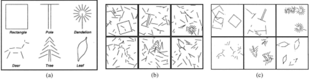
The first set of tests uses the six models shown in Fig­ ure 2a. To create datasets D, model segments are ran­ domly scaled and placed in the data images. In addi­ tion, the model line segments are fragmented, skewed and potentially omitted. Finally, random clutter and struc­ tured clutter are added to the data. Structured clutter con­ sists of more highly degraded copies of the same object model. Examples are shown in Figures 2b and 2c. This dataset and results for it are available through our website (http: I /www. cs. colostate. edu/ -vision/ ).

A second set of tests use data images with 50 randomly placed segments. Models are created by randomly drawing 5, 10, 15 or 20 of these segments. This dataset tests the reliabil­ ity of the proximity heuristic as the ratio of model to clutter lines varies.

5.1 Six Corrupted Models

The models shown in Figure 2a exhibit characteristics known to make matching difficult. For example, the Pole is an inter­ esting case for the key feature algorithm because of its sim­ plicity: there exists only one possible model triple for the key feature algorithm to exploit. The Dandelion exhibits a 16 fold near symmetry; model symmetry complicates matching for many well established techniques [Grimson, 1990]. The Leaf presents an example where model and data line segments ap­ proximate a curved contour. For this model, a many-to-many mapping between model and image features is needed to ac­ count for breakpoints at different positions along the curve.

A Monte Carlo simulator produces corrupted image data. The simulator rotates, translates and scales the model so placement and size are unknown. Model segments are also fragmented and skewed. In 24 of the problems, 0, 10, 20 and 30 additional clutter segments are randomly placed about the image. A sampling of this data is shown in Figure 2b. In the other 24 problems, 0, 1, 2 and 3 additional corrupted model instances are added. A sampling of this data is shown in Fig­ ure 2c.

The steepest-descent local search algorithm has been run for 1, 000 trials on all 48 problems. The key feature algorithm has been run using the best n triples. The resulting run times and quality of results are indicated in Figure 3a. Problem in­ stances are grouped along the x axis by model type, with run time plotted on they axis. Those problems where key features fai led to find the optimal match are indicated in the separated band at the top of the plot.

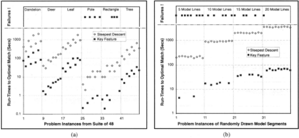
Two critical types of information are conveyed by this plot. First, over 1, 000 trials, the random starts algorithm never failed to find the optimal match at least once. Conversely, the key feature algorithm failed in 7 out of the 48 cases. Sec­ ond, the key feature algorithm is dramatically more efficient in terms of run time, typically taking less than 1/10th of the time required by the random starts local search algorithm.

The key feature algorithm fails on the simpler object mod­ els: the pole and rectangle 1 · Two factors may explain these failures. First, simulator fragments model line segments with a fixed probability per unit length. Hence, longer segments fragment more. The rectangle and pole have the longest individual segments, and therefore the highest degree of fragmen­ tation. Too much fragmentation prevents the proximal triples algorithm from finding triples which participate in the best match. The second factor is that there are fewer total features on the simpler models, further reducing the opportunities for the algorithm to find a good key feature .

1 On symmetric models such as the rectangle and building in Fig­ ure I, symmetric matches are treated as equivalent.

The statement that the local search algorithm did not fail requires some elaboration. Based upon the 1, 000 trials, the probability of success P. has been estimated for each individ­ ual problem. Using these estimates, it is more proper to say that the required number of trials to find the best match with 95% confidence, t. from equation 6, never exceeds 1, 000.

Actually, far fewer than 1, 000 trials are required for most of the problems in the test suite. Less than 100 trials are re­ quired for 33 out of the 48 problems, and only 3 problems re­ quire more than 500 trials. Likewise for the key feature al­ gorithm, it is typically not necessary to consider all n triples.

The run times shown in Figure 3a are intentionally conserva­ tive, making no assumption that there is a priori knowledge of how hard a specific problem is to solve.

Looking at the actual work needed per problem, the key fea­ ture algorithm finds the best match from the first ranked triple in 26 out of the 48 cases. There are 7 cases where a triple in the top 50 leads directly to the best match. Finally, in the 8 remaining cases, simply running the steepest-descent algo­ rithm where only pairs are added misses the best match. How­ ever, in these cases, the final application of random starts local search locks onto the globally best match. This is counted as a success for the key feature algorithm.

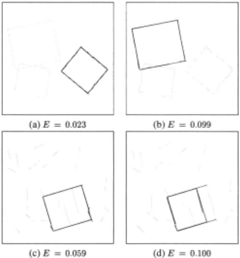
It is interesting to observe how the key feature algorithm is lead astray. Figure 4a shows the optimal match found by ran­ dom starts local search for the three rectangles problem. Fig­ ure 4b shows the best match found by the key feature algo­ rithm. This is the 2nd best match found by the local search algorithm. Figure 4c shows the optimal match found by ran­ dom starts local search for the case of 20 random clutter lines. Figure 4d shows the best match found by the key feature al­ gorithm: again, it is the 2nd best match found by local search. This case is interesting because the coincidently placed long clutter line creates a 'false' rectangle which traps the key fea­ ture algorithm.

5.2 Randomly Placed Lines

The probability that the key feature algorithm will succeed depends upon the likelihood that a triple f in F belongs to the best match c*. This likelihood, in turn, depends upon the probability that the two segments closest to a data segment co­ incide with the two closest segments in the model. As the re­ sults above suggest, this is a good but not perfect heuristic.

One way to think about this likelihood is to consider how the ratio of clutter to model features varies as more or fewer segments are drawn from a fixed size set of data segments. To illustrate, a set of 40 test problems has been generated, each with 50 randomly placed non-intersecting line segments. Ten distinct sets of 50 random segments are used, and models are created by randomly selecting 5, 10, 15 or 20 from each set.

The results for these 40 problems are shown in Figure 3b. They support the hypothesis that a higher clutter ratio causes the key feature algorithm to become unreliable. The key fea­ ture algorithm fails on 8 out of 10 of the 5-segment models, while only failing on 1 out of 10 for the 20-segment models.

Because the local search algorithm does not depend upon key features, we do not expect it to have difficulty with these problems. Figure 3b shows that this is in fact the case, with lo­ cal search solving all40 problems reliably in less than 1, 000 trials. Moreover, it may surprise some readers to know that the average t. for 95% confidence decreases as these models get larger. For the problem instances with models of 5 seg­ ments, t~ = 122.3, while for the models of 20 segments t~ = 74.2. A t-test on this data indicates that the drop is statistically significant: t = 5.03 and p ::=; 0.001. While far fewer than 1, 000 trials are actually needed, for the sake of consistency, the times reported in Figure 3b are all based upon 1, 000 trials.

5.3 A Real World Example

It should now be apparent that the key feature algorithm has profound computational advantages over random starts local search. When it succeeds, it requires one to two orders of magnitude less computation. Real world examples can be found where it works well, including many of the fairly clean 2D line matching problems common in the literature.

Let us now consider a very difficult problem, the building shown in Figure 1. There are 4 model line segments and 443 data segments, generating 1, 772 possible pairs of segments. More important in terms of problem difficulty, there are multi­ ple instances of buildings interacting with other buildings and roads, creating a combinatorial explosion of possible partial matches. Also, the globally best match 2 is highly fragmented and must be pieced together by a search algorithm before it appears more attractive than many of the other more obvious partial rectangles.

To fully test random starts local search on this problem, 10, 000 trials have been run. The best match is found in only 12 of these trials: the estimated probability of success P. =

2 Strictly speaking, we do not know the match shown in Figure ld to be the global optimum. However, through extensive study of this problem and our ability to eye-ball the results, we are relatively cer­ tain it is best.

0.0012 is tiny. Required trials t. = 2, 494 and average time to run a trial is 24 seconds. Consequently, local search re­ quires nearly 18 hours to reliably solve this problem.

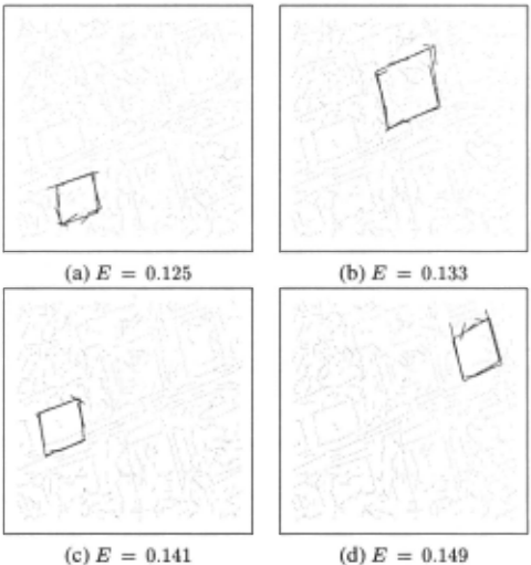
While random starts local search has allowed us to find this best match, 18 hours is far too much time for any practical on­ line system to spend looking for one building. In contrast, the key feature algorithm is very fast, completing in a matter of minutes. However, it fails to find the best match. Instead, it finds the match shown in Figure Sa. This is not totally uninter­ esting, since according to the local" search algorithm, this is the second best match in the image. However, it has a markedly larger match error: 0.125 as opposed to 0.101 for the global optimum. Local search also, in some sense, finds two other buildings: Figures 5c and 5d show the fourth and fifth ranked matches. Figure5b shows that the third ranked match is a vari­ ant on the global optimum, sharing many of the same features.

6 Conclusion

We have presented a variant upon key feature matching. It operates within an optimal matching framework and uses the same criterion function to rank both key features and final ob­ ject model matches. On controlled problem sets, it has been shown that the underlying proximity heuristic yields key fea­ tures which allow an algorithm to quickly find many but not all optimal matches. In an example of the cost versus gener­ ality trade-off typical in Artificial Intelligence, random starts local search is shown to be both more robust and more com­ putationally demanding.