
An Approximate 0-1 Edge-Labeling Algorithm for Constrained Bin-Packing Problem
Proceedings of the Fifteenth International Joint Conference on Artificial Intelligence. Search. Pages 1402-1410.
© 1997 International Joint Conferences on Artificial Intelligence
Abstract
This paper describes a constrained bin-packing problem (CBPP ) and an approximate, anytime algorithm for solutions. A CBPP is a constrained version of the bin-packing problem, in which a set of items allocated to a bin are ordered in a way to satisfy constraints defined on them and achieve near-optimality . The algorithm for CBPP uses a heuristic search for labeling edges with a binary value, together with a beam search and constraint propagation. Some experimental results are provided. This algorithm has been successfully applied to industrial-scale scheduling problems.
- [Garey and Johnson, 1979] Michael Garey and David Johnson. Computers and Intractability, A Guide to the Theory of NP-Completeness. W. H. Freeman and Company, 1979.
- [Knuth, 1975] D. Knuth, Estimating the efficiency of backtracking programs, Mathematics of Computation 29, No. 129, pages 121-136, 1975.
- [Dean and Boddy, 1988] T. Dean and M. Boddy, An analysis of time-depending planning, Proceedings of the 7th National Conference on Artificial Intelligence, pages 49-54, 1988.
- [Lawler et al., 1985] E. Lawler, J. Lenstra, A. Rinnooy and D. Shmoys, The Traveling Salesman Problem: A Guided Tour of Combinatorial Optimization, John Wiley and Sons, 1985.
- [Martello and Toth, 1990] S. Martello and P. Toth, Knapsack Problems: Algorithms and Computer Im- plementations, John Wiley & Sons, 1990.
- [Eilon and Christofides, 1971] S. Eilon and N. Christofides, The loading problem, Management Science 17, pages 259-267, 1971.
- [Hung and Brown, 1978] M. Hung and J. Brown, An algorithm for a class of loading problems, Naval Re- search Logistics 25, pages 289-297, 1978.
- [Nilsson, 1980] N. Nilsson, Principles of Artificial Intel- ligence, Tioga Press, 1980.
- [Winston, 1984] P. Winston, Artificial Intelligence (sec- ond edition), Addison-Wesley, 1984.
- [Vollman et al., 1992] T. Vollman, T. Berry and D. Whybark, Manufacturing Planning and Control Sys- tems, Irwin, 1992.
References were extracted automatically from the PDF and may contain errors.
Full text extracted automatically from the PDF; figures, tables and equations may differ. The PDF is the version of record.
1 Introduction
We can see many instances of the bin-packing problem (BPP) which is characterized as follows: Given a finite number of bins whose sizes are the same, and a finite set of items whose size is no more than the bin size, find a partition of the items into disjoint subsets such that the sum of the sizes of the items in each subset is no more than the bin size, and such that the number of the bins used is as small as possible. This bin-packing problem is NP-hard (Garey and Johnson, 1979; Martello and Toth, 1990).
The manufacturing and process industries often need to create production units consisting of subunits that are identical with respect to some criteria. These pro duction subunits are normally called groups, batches, or lots [Vollman et al., 1992). When creating such groups we frequently face problems that can be considered par ticular instances of the constrained bin-packing problem (CBPP), which has additional restrictions over the bin packing problem in that items in each group have to be sequenced satisfying all given constraints, creating ordered groups. In addition to satisfying all the con straints, items in each bin should be ordered in a way to minimize primarily the number of bins and secondly aggregate cost.
Consider an example of a production scheduling prob lem from the steelmaking industry. Given a number of orders (items) from customers, production schedules are created by grouping the orders by considering many at tributes such as chemical composition, process routing and delivery due date. At the melt shop large bins called converters are used to transform molten iron into puri fied molten steel. A converter typically contains a max imum of 250 tons. A group of orders in the converter is called a heat. For the production of the same set of orders, some groupings require fewer heats to be made than other groupings due to better utilization of the con verter. This is desirable because there is a high fixed cost associated with processing a heat that is independent of the size of the heat. Hence, one of the primary goals in steelmaking scheduling is to minimize the number of heats at the melt shop required to produce all of the given orders. This problem description alone is similar to BPP.
Yet another issue is the production cost which is in curred when producing one order after another. Due to the characteristics of subsequent processes such as cast ing and rolling, even for two solutions with the same number of heats, the total cost of producing all orders may be different depending on the sequence of orders within each heat. Therefore, a secondary goal is, for the same number of heats, to find the sequences of or ders within individual heats that minimizes the aggre gate production cost. With this secondary requirement, the problem becomes CBPP.
For the exact solution of ordinary (unconstrained) BPP, very little can be found in the literature [Eilon and Christofides, 1971; Hung and Brown, 1978), and they can solve only small size instances. We can find approximate algorithms of BPP in the literature, a few of which include First Fit, Best Fit, First Fit Decreas ing, and Best Fit Decreasing [Garey and Johnson, 1979; Martello and Toth, 1990).
In ordinary BPP, we can choose any item to fill a bin from the item pool. In contrast, in CBPP, the next item to choose from is limited to a subset of the item pool whose elements can feasibly be inserted into the bin. Whereas many reports on the ordinary BPP algorithm are available, to the best of our knowledge, no literature on algorithms regarding the CBPP exists.
A directed graph with all of its edges labeled uniquely determines a solution. Possible labels associated with each edge is binary: 1 (selected) or 0 (discarded). In this paper, we "present an approximate algorithm for CBPP that finds near-optimal solutions in a reasonable amount of time. We call this algorithm an approximate 0-1label ing algorithm. Given a directed graph constructed from a CBPP, the 0-1 labeling algorithm labels all edges as either 1 or 0 until exhausted. in an incremental way, re sulting in a set of ordered groups. Heuristic information such as the topological structure of graphs is used in se lecting edges to label. This algorithm was developed at IBM T.J. Watson Research Center as a means to solve large-scale industry grouping and scheduling problems. It is currently used in several real-world applications.
The remainder of this paper is organized as follows. In the next section, the problem statement is given. In Sec tion 3 we present an approximate algorithm for CBPP in detail. We then provide experimental results together with some analysis.
2 Problem Statement
The following is an abstraction of CBPP.
We are given a finite set of items, each of which has a size. An ordered group is an ordered sub set of those items. The total weight of the or dered group cannot exceed the bin capacity. If two items i,. and im are adjacent in the bin, we incur a cost from im to i,., which is not nec essarily the same as a cost from i,. to im, and which may be infinite, implying that the solu tion is infeasible. The primary goal is to cre ate a feasible solution with minimum number of ordered groups. When two solutions have the same number of ordered groups, the one with the minimum aggregate cost is preferred.
CBPP can be considered a combined version of the bin-packing problem and the traveling salesman problem (TSP) because the bins have a fixed capacity, items in a bin are ordered, and we wish to minimize the aggregate cost. Furthermore, when an item, ik, is assigned to a bin, only a subset of the unassigned items which could follow ik can be placed in the same bin.
In general, we can put any number of constraints on the problem. Some examples of the constraints fre quently encountered in industrial search problems are:
- items of type A can not follow items of type B or E in a bin
- two different items of type C within a bin should be separated by some number of items with an aggre gate size of at least s
- the aggregate size of items of typeD in a bin cannot exceed s
- the number of items of the same type in a bin is limited to n
Note that the first constraint is a local constraint be tween two adjacent items, while the rest are non-local constraints.
3 An Approximate Algorithm for CBPP
In this section, we present the underlying data struc ture, the CBPP graph, a heuristic that aids in solving the CBPP, and the detailed description of the 0-1 edge labeling algorithm, an approximate algorithm for CBPP.
3.1 CBPP Graphs
The problem space of a CBPP can be represented by a directed graph, G(V, E), where Vis a set of vertices and E is a set of directed edges. Initially, each item i,. in CBPP is mapped to a vertex v, in V. So, the number of items in CBPP is the same as lVI· A directed edge e(vi,vj) in E incidents from Vi (tail) to Vj (head). Each directed edge e is assigned a non-negative cost c( e) and represents a valid path from the tail vertex to the head vertex with an associated cost. By valid, we mean that the sum of the sizes of the items associated with the vertices does not exceed the bin capacity, and that the sequencing from the tail vertex to the head vertex does not violate any constraints defined between the two. In general, there may be a number of constraints defined between two vertices, as was seen from the examples of the constraints in the previous section.
A CBPP graph is usually incomplete, and, in many cases, it is quite sparse because of many constraints among the vertices. This is the difference between the problems we are dealing with and the optimization prob lems such as the ordinary BPP, which is fully connected with uniform cost, and the symmetrical traveling sales man problem [Lawler et al., 1985], where no constraints are imposed on edges. 1
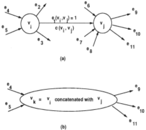
As search (labeling) proceeds, lVI of a CBPP graph is decreased as a result of concatenation of two vertices, creating a new vertex (ordered group), as shown in Fig ure 1.
Note that a vertex represents either an original atomic vertex (an item) or an ordered group which is a sequence of items. An initial CBPP graph represents a solution where the number of bins is equal to the number of ver tices. Obviously, it is not a good solution. Two adjacent vertices connected by an edge labeled as 1 are concate nated.
An ordered group for each bin in a CBPP is conceptu ally equivalent to a sequence of vertices concatenated with edges, where the total size of an ordered group should not exceed the bin capacity. Therefore, the CBPP can be regarded as a search that labels edges so as to minimize the number of ordered groups with the mini mum aggregate cost. The problem is to find a labeling of edges.
1 Note that the CBPP graph is different from the con straint graph (or network) usually referred to in AI. In the constraint graph, each node represents a variable having its own domain values, and each edge bears a set of constraints between the two values of the two variables.
3.2 Heuristics
Finding an optimal set of ordered groups is computation ally intractable. To cope with this problem and to pro duce near-optimal solutions search heuristics are used. Using heuristic information often has a significant im pact on the performance of search algorithms. In the CBPP solution, a heuristic based on topological struc ture is used in selecting edges to label. In addition, a beam search and constraint propagation techniques are exploited to prune the search space.
An abstraction of a search problem is a search tree. The nodes of the tree represent the states, and the links of the tree represent the operators. A state represents a subset of the whole search space. In CBPP, each labeling of an edge in the graph corresponds to an execution of an operator, which in turn changes one state to another.
The search starts from the root node with an initial CBPP graph. Then, from the current CBPP graph, we collect all edges and rank them according to predeter mined heuristics. During the search, an ordered groups are dynamically created by concatenating two vertices with an edge in the current CBPP graph. Optimality of the solution is dependent on which edges are selected and labeled during the search.
The heuristic used for selecting which edges to label is based on the topological structure of the CBPP graph. The urgency of edge e( Vi, Vj) is defined as the smaller of out-degree( Vi) and in-degree( Vj ). For example, in Figure
1( a), the urgency of e1 (vi, Vj) is 3, which is the smaller of 3 (out-degree of vi) and 4 (in-degree of Vj ). The urgency represents the possibility that either vertex Vi or Vj loses the chance to grow (resulting in a deadlock). Intuitively, the fewer e's sibling edges exist, the higher its chance to be selected would be. This topological heuristic helps the algorithm to find the minimum number of ordered groups, where a single item is regarded as one ordered group.
In addition to the urgency, we may use other heuris tics on both domain-dependent and domain-independent information.
3.3 0-1 Edge-Labeling Algorithm
Initially all the edges in the CBPP graph are unlabeled, but they are eventually labeled as either 0 or 1. The labeling algorithm derives a set of ordered groups by incrementally labeling a selected edge as 0 (discarded) or 1 (selected) until all edges are completely labeled. When an edge is labeled as 1, we have a new ordered group concatenating two vertices connected by the edge; and, the two existing ordered groups being concatenated are discarded.
From the viewpoint of the search space, labeling an edge e as either 0 or 1 partitions the solution search space into two: one including solutions with e labeled as 1 and the other including solutions with e labeled as 0. The labeling algorithm incrementally modifies an initial CBPP graph to one with more number of edges labeled. The algorithm is basically a depth-first search. The detailed procedure of the 0-1 edge-labeling search follows. In this description, G N (V, E) denotes a CBPP graph associated with search node N.
0-1 Edge-Labeling Algorithm
- Initialize solutions and open_nodes to the empty set and create the root node as node N of the search tree.
- Sort all unlabeled edges e E E at GN(V, E) in terms of edge selection heuristics.
- Push the best beam_width number of edges onto besLedges(N).
- Pop the the first edge, e(vi,vj), from besLedges(N), and label it as 1. If best_edges(N) is still non-empty, then push N onto open_nodes.
- Create a new search node S, a child node of N, and generate the new CBPP graph Gs(V, E) from GN(V,E). Label e(vi,vj) in Gs(V,E) as 1. For the new child node S:
- Concatenate the two items (or ordered groups) Vi and Vj, creating a new ordered group. Remove Vi and Vj from S and add the new ordered group (Vi, Vj) to S.
- Each of the edges in the current CBPP graph G s (V, E) is evaluated and those which no longer satisfy all relevant constraints are la beled as 0 and removed 2 ·
- If any edges in G s ( V, E) are unlabeled, set N = S and go to Step 2, otherwise continue with Step 6.
- Induce the solution s from S and evaluate. If s can be considered a member of the set of best solutions discovered so far, store s in solutions.
- If open_nodes is not empty and we need a better solution or additional solutions, and if we have not exceeded the maximum number of search it erations, pop the top node N from open_ nodes and go to Step 4. Otherwise exit with solutions.
Notes:
- Step 1 (initialization): Generated solutions (sets of ordered groups) will be kept in solutions. Intermedi ate search tree nodes that can be further expanded for alternative search branches will be pushed onto the stack open_nodes.
- Step 5a (creation of a new search node): As an example, consider Figure l(a), where edge e(vi,vj) is being labeled as !(selected). Then, as can be seen in (b), vertices Vi and Vj are concatenated and a new vertex (ordered group) vk is created.
As a result of this step, the number of ordered groups in the new search node is always one less than that of its parent search node. In general, if we start the search with n ordered groups then it is reduced to n - k at the k-th search level with the level of the root node defined as 0.
- Step 5b (labeling inconsistent edges as 0): Here, constraint propagation is effectively used in pruning the search space, and finding the termina tion of the search tree. For example, again consider Figure l(b). As a consequence of labeling of e1 as 1, five incident edges ez, e3 , es, e7 and e8 are la beled as 0 {discarded). In addition, some of edges ( e4, e5, eg, e1 0, e1l) not yet labeled may be labeled as 0 as a result of constraint checking in this step.
Note that the heuristics employed in the labeling search focus on the selection of an edge to label, in stead of on the selection of a node to expand. Since the goal state is neither unique nor explicitly given it is practically impossible to compute a heuristic evaluation function that estimates of the cost of reaching the goal state from the current search node [Nilsson, 1980].
2 1n practice, only those edges topologically connected to the committed edge, as well as those edges selected using the topological heuristic, are evaluated.
3.4 More on 0-1 Edge-Labeling
The worst case · space and time complexity of the 0-1 edge-labeling search are O(n) and O(bn), respectively, where b is the branching factor (the beam width in our case) and n is the number of items. Notice that the worst case depth of the search tree is n - 1. As described in the algorithm, the algorithm only needs to store a stack of the nodes on the search path from the root to the current search node; hence, the memory requirement is only linear in the number of items (or the search depth). In contrast, in situation where the branching factor is large, the time complexity of the search algorithm expo nentially grows with the search level. Therefore, limiting the branching factor (beam width) is crucial to the per formance.
One possible drawback of using beam search is that we might miss a path in a node expansion which really is the best choice. As a result, a naive adoption of the beam search may yield bad solutions [Winston, 1984]. How ever, we mitigate this drawback of the beam search in the proposed edge-labeling algorithm. Using edge-labeling, we can construct an identical ordered groups (sequence) in many different ways since the edges included in the ordered group are consistent and independent one an other. For example, there are 5! = 120 different ways to construct a particular ordered group with 6 vertices (5 edges). In order words, in the situation where even if the truly second best edge e2 , instead of the truly best edge e1, is selected for some reason at the current search level, it is highly likely that e1 is selected on the next level.
In addition to the apparent savings of computational resources, exploiting beam search enables quick navigat ing in the solution space, which is essential to find a near-optimal solution within a limited amount of time. In the traditional algorithms for instantiating variables, it is not easy to quickly move around the search space since they basically rely on backtracking [Knuth, 1975]. Although it is possible to use the beam search in this kind of search, it is not possible to recover from miss ing variable assignments once performed. In the edge labeling algorithm, however, it is possible without expe riencing such a problem. By limiting the beam width, we can quickly move around the search space. As an ex treme case, if we set the beam width to one, each branch from the root node results in a single solution and every solution is likely to be different from the rest.
4 Experiments
The 0-1 edge-labeling algorithm for CBPP was imple mented in the C++ programming language under AIX on an RS/6000 39H workstation with 256MB of memory. To test the algorithm, we generated several problems by varying the number of items and the sparsity of the ini tial CBPP graph. The sparsity is defined as the ratio of the actual number of edges in the graph with finite cost to the number of edges in a complete directed graph with the same number of vertices. The size of each item was set to a positive random value less than the bin size. The cost incurred when one item is placed adjacent to another was determined by a square matrix of positive random values.
For the experiments we used the urgency measure as the primary rule in selecting an edge from among the unlabeled edges. If multiple edges were chosen based on this measure, then the cost of the edges was used as a tie-breaker.
The goal is to find the minimum number of ordered groups with the minimum aggregate cost. However, as previously stated, finding a near-optimal solution in a reasonable amount of time is often more important than finding a truly optimal solution. Accordingly, we stopped each search after ten minutes elapsed time and examined the set of solutions that had been generated.
To provide an insight on the 0-1 edge-labeling algo rithm, we also generated results using the best-fit de creasing (BFD) algorithm, which is one of the best ap proximate algorithms for BPP [Martello and Toth, 1990]. In the BFD, all the items are sorted in a decreasing or der of size, and an item with lower index is considered first. A bin which can accommodate the item with mini mum residual capacity is used for packing. Although the BFD algorithm is for BPPs we believe that the results of it can be a reference when evaluating the results of the 0-1 edge-labeling algorithm. The results are summarized in Tables 1-5. In those tables, the second column ("bins, CBPP") denotes the number of bins, and the third col umn ("cost, CBPP") denotes the aggregate cost of all ordered groups in a solution. Note that a solution with a bigger aggregate cost is better than another solution with a smaller aggregate cost , if the number of bins of the former is less than that of the latter.
The time for the BFD heuristic was negligible and is not shown. Since the BFD heuristic only attempts to find a feasible solution and does not minimize the aggre gate cost, the cost for the BFD solution is not shown.
We note that the 0-1 edge-labeling algorithm found good solutions to the problem. With respect to the num ber of bins used, the 0-1 edge-labeling algorithm did well except when the sparsity was unity while the number of items was large. The reason that BFD's result is better than that of the 0-1 edge-labeling algorithm in the case the sparsity is close to unity or the number of items is large is that the run time is limited to ten minutes (so, only a small portion of the search space is investigated). On average, the 0-1 edge-labeling algorithm yielded solu tions which used 22% fewer bins than the BFD heuristic.
Figure 2 shows the progression ofthe 0-1 edge-labeling algorithm for a graph with 64 items and sparsity 0.500. The time for the 0-1 edge-labeling algorithm is the time when the indicated solution was generated. The 0-1 edge-labeling algorithm found, after 11 seconds, a so lution that used 10 bins which is already better than the 11 bin solution found using the BFD heuristic. Be tween 11 and 12 seconds, the 0-1 edge-labeling algorithm found a lower cost solution using 10 bins and then a so lution with 9 bins. Between 12 and 40 seconds, the algonumber or bins rithm reduced the path cost at 9 bins from 441 to 367. This anytime [Dean and Boddy, 1988] behavior of the 0-1 edge-labeling algorithm is very useful in industrial problem solving.
| sparsity | bins, CBPP | cost , CBPP | bins, BFD |
|---|---|---|---|
| 0.050 | 10 | 687 | 17 |
| 0.100 | 6 | 690 | 13 |
| 0.500 | 4 | 387 | 6 |
| 1.000 | 3 | 377 | 3 |
| sparsity | bins, CBPP | cost, CBPP | bins, BFD |
|---|---|---|---|
| 0.005 | 43 | 575 | 49 |
| 0.010 | 33 | 1185 | 43 |
| 0.050 | 14 | 1181 | 26 |
| 0.100 | 10 | 1028 | 17 |
| 0.500 | 8 | 529 | 10 |
| 1.000 | 7 | 790 | 7 |
| sparsity | bins, CBPP | cost, CBPP | bins, BFD |
|---|---|---|---|
| 0.001 | 107 | 1154 | 119 |
| 0.005 | 79 | 2232 | 95 |
| 0.010 | 58 | 2280 | 86 |
| 0.050 | 23 | 2344 | 38 |
| 0.100 | 19 | 1318 | 28 |
| 0.500 | 18 | 885 | 21 |
| 1.000 | 17 | 2169 | 17 |
| sparsity | bins, CBPP | cost, CBPP | bins, BFD |
|---|---|---|---|
| 0.001 | 205 | 2351 | 229 |
| 0.005 | 109 | 5099 | 158 |
| 0.010 | 73 | 5430 | 126 |
| 0.050 | 41 | 2956 | 65 |
| 0.100 | 40 | 1613 | 51 |
| sparsity | bins, CBPP | cost, CBPP | bins, BFD |
|---|---|---|---|
| 0.001 | 338 | 8434 | 410 |
| 0.005 | 145 | 10918 | 247 |
| 0.010 | 115 | 9032 | 185 |
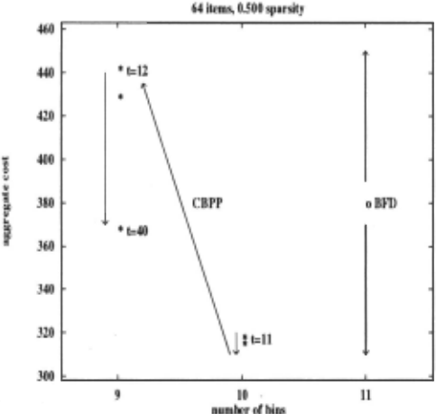
Figure 2: Progression of the 0-1 edge-labeling algorithm. It is an anytime algorithm and it is shown that bin us age and aggregate cost are further optimized as search proceeds.
5 Conclusion
We have defined a class of problems called constrained bin-packing problems which characterizes many fre quently encountered industrial scheduling problems. Be cause no known existing techniques can effectively solve this class of problems, we have developed a CBPP al gorithm which is based on an approximate 0-1 edge labeling.
We believe that this technique meets most of the in dustrial requirements in term of time, space and quality. For difficult search problems, many near-optimal solu tions can be found where previously even a single solu tion was considered difficult, if not impossible, to obtain, and most importantly, the algorithm can find these near optimal solutions in a reasonable amount of time.
However, as with any technique, there is a limit to the scope of its application. We consider the CBPP solution technique inappropriate for unconstrained problems such as the simple traveling salesman problem for which there exist other techniques that yield better solutions in less time.
The approximate 0-1 edge-labeling algorithm for CBPP described in this paper has been successfully applied to industrial grouping and scheduling problems.
Acknowledgments
We would like to thank Jayant Kalagnanam and Richard Goodwin for their valuable comments on the draft of this paper.
@inproceedings{ijcai1997p202,
  title     = {An Approximate 0-1 Edge-Labeling Algorithm for Constrained Bin-Packing Problem},
  author    = {Lee, Ho Soo and Trumbo, Mark},
  booktitle = {Proceedings of the Fifteenth International Joint Conference on
               Artificial Intelligence, {IJCAI-97}},
  publisher = {International Joint Conferences on Artificial Intelligence},
  editor    = {Martha E. Pollack},
  pages     = {1402--1410},
  year      = {1997},
  note      = {Search},
  url       = {https://ijcai.org/proceedings/1997/202},
}
TY - CPAPER TI - An Approximate 0-1 Edge-Labeling Algorithm for Constrained Bin-Packing Problem AU - Lee, Ho Soo AU - Trumbo, Mark T2 - Proceedings of the Fifteenth International Joint Conference on Artificial Intelligence, IJCAI-97 PB - International Joint Conferences on Artificial Intelligence PY - 1997 SP - 1402 EP - 1410 UR - https://ijcai.org/proceedings/1997/202 ER -Copied
Machine-readable versions of this paper, for tools and AI agents:





