
PRISM: A Language for Symbolic-Statistical Modeling
Proceedings of the Fifteenth International Joint Conference on Artificial Intelligence. Probabilistic Reasoning. Pages 1330-1338.
© 1997 International Joint Conferences on Artificial Intelligence
Abstract
We present an overview of symbolic-statistical modeling language PRISM whose programs are not only a probabilistic extension of logic programs but also able to learn from examples with the help of the EM learning algorithm. As a knowledge representation language appropriate for probabilistic reasoning, it can describe various types of symbolic-statistical modeling formalism known but unrelated so far in a single framework. We show by examples, together with learning results, that most popular probabilistic modeling formalisms, the hidden Markov model and Bayesian networks, are described by PRISM programs.
- Asai et al. 93)
- Asai,K., Hayamizu,S. and Handa,K., Prediction of protein secondary structure by the hidden Markov model, CABIOS 9 No.2 pp141-146, 1993.
- Charniak,E., Statistical Language Learn- ing, The MIT Press, 1993.
- Charniak et al. 93)
- Charniak,E. and Goldman,R.P., A Language for Construction of Belief Networks, IEEE PAMI 15 No 3, pp196-208, 1993
- Hashida 94
- Hashida,K., Dynamics of Symbol Systems, NGC 12, pp285-310, 1994.
- Muggleton
- Muggleton,S., Inductive Logic Program- ming, NGC 8, pp295-318, 1991.
- Ng,R. and Subrahmanian,V.S., Probabilistic Logic Programming, Information and Computation 101, pp150-201, 1992.
- Pearl
- Pearl,J., Probabilistic Reasoning in Intelli- gent Systems, Morgan Kaufmann, 1988.
- Poole
- Poole,D., Probabilistic Horn abduction and Bayesian networks, Artificial Intelligence 64, pp81- 129, 1993.
- Rabiner
- Rabiner,L.R., A Thtorial on Hidden Markov Models and Selected Applications in Speech Recognition, Proc. of the IEEE 77, No. 2, pp257- 286, 1989.
- Sato,T., A Statistical Learning Method for Logic Programs with Distribution Semantics, Proc. of ICLP 95, pp715-729, 1995.
- Tanner,M., Tools for Statistical Inference (2nd ed.), Springer-Verlag, 1986.
References were extracted automatically from the PDF and may contain errors.
Full text extracted automatically from the PDF; figures, tables and equations may differ. The PDF is the version of record.
1 Introduction
We can make programs probabilistic by incorporating probabilistic elements, which is rather obvious. What is less obvious would be the existence of a general learn ing algorithm for these probabilistic progr~ms. I~ ~his paper, we present an overview of sy~bohc-stat~st~cal modeling language PRISM (PRogrammmg In Statistical Modeling). PRISM was born as the _integrati?n of lo?ic programming and the general l~arnmg ~lgonthm w1t~ which programs can change thetr beha:wrs, a posten ori, by learning from examples. PRISM ts a_new t~p~ of programming language designed for symbohc-stattsttcal modeling of complex objects and the real world.
The theoretical basis of PRISM is fixed point (least model) semantics and probability theory, but the de velopment was spurred by the noticeable success of HMM (hidden Markov model) in speech recognition (and their applications to genetic information processmg) [Rabiner 89, Asai et al. 93], a rapid surge of the interest in statistical methods in NLP (Nat ural Language Pro cessing) [Charniak 93], well-developed uncertainty han dling mechanisms in Bayesian networks [Pearl 88] and very encouraging results from ILP (Inductive Log~c Pro gramming) [Muggleton 91]. They are all symbohc sys tems able to learn from statistical data.
*This paper is partly based on a report submitted for Computational Logic Network news letter.
t email: sato@cs. titech.ac.jp
t email: kame@cs. titech.ac.jp
PRISM offers a common vehicle for these diverse re search fields in symbolic-statistical modeling, and also gives us hopes for building even more complex and intel ligent systems. This is because PRISM programs ca~ be arbitrarily complex (no restriction on the form or stze), and what is more, regardless of the complexity, there is at least in theory, a method for PRISM programs to le~rn from positive/negative examples. To put it differ ently, we have the possibility of training arbitrarily large programs so that they behave as we desire.
In the rest of paper, we describe PRISM in stages. We first describe the semantic aspect of PRISM programs in Section 2, then move to an example in Section 3 where a program modeling human blood types is presen~ed. Sec tion 4 explains learning and the EM (Expectatwn Max· imization) algorithm. PRISM as a programming system is described in Section 5, followed by examples of the hidden Markov model and Bayesian networks in Section 6. Section 7 contains related work and Section 8 conclu· SlOn.
2 PRISM programs and distributional semantics
PRISM programs are roughly defined as logic programs with a probability distribution given to facts. So we can compute any recursive functions as a special case of non probabilistic facts. To capture PRISM programs mathe matically however, we need a probabilistic generalization of fixed point semantics.
A PRISM program DB is a set of definite clauses writ ten as DB = FUR where F is a set offacts (unit clauses) and R is a set of rules (non-unit clauses). In the theo retical setting, we always equate clauses with the set of their ground instances, and allow DB to be countably infinite.
What makes PRISM programs differ from usual logic programs is a basic joint probability distribution PF given to F. It means that ground unit clauses A1, A2, ... be longing in F are probabilistically true and the probabil ities are determined by the joint probability distribution Pp like Pp(A1 = 1, A2 = 0, ... ) = 0.3 etc. Here we con sider ground unit clauses as random variables taking 1 (true) or 0 (false).
Sampling from Pp determines the set of true facts F', and the least model of F' U R determines the truth of all ground atoms appearing in the original program. On the basis of this observation, we extend Pp to a joint probability distribution Poa for all (ground) atoms ap pearing in DB. We define the denotation of DB as P08 and call it distributional semantics. Formal treatment of distributional semantics is found in [Sato 95] where the existence of a joint probability distribution for infinitely many random variables and the measurability of the set of least models are discussed.
We illustrate how we can extend Pp to Poa by giving a small example. Let {A1, A2} U {B1 + AI,BI +- A2,B2 +- A2} and Pp(A1 = xi,A2 = x2) be a program and the associated basic distribution respec tively. Suppose we got a sampling from Pp which was (AI = 1, A2 = 0) in vector notation i.e. the set of true facts is {AI}.
Imagine then a new program {AI} U {B1 +- A1, B1 + A2,B2 +- A2} and its least model {A1,BI}. This model determines the truth of B1 and B2 as (B1 = 1, B2 = 0). In this way, B1 and B2 become random variables via the least model, and a truth value vector (x1, x2) for (AI,A2) sampled from Pp uniquely determines the truth value vector (y1 , Y2) of (B1 , B2). We denote this func tional relationship by rp DB ((xi, x2)) = (YI, Y2). Then PDa(BI = YI, B2 = Y2) is calculated by It' DB from Pp as follows. 1
In the learning phase, as seen in Section 4, we read the above equation the other way around, and adjust Pp to maximize PDa(Bl = Y1,B2 = Y2), the probability of producing what we observe.
3 A blood type example
As a typical symbolic-statistical model, we present a blood type program. It is very like a Prolog program and as usual, variables begin with upper case letters. We hope that the following comments will help the reader understand the program.
- This program describes how one's blood type (bloodtype/1) is determined from the genes in herited from the parents. It happens to be non recursive but there is no problem in writing recur-
1 This equation says, in the case of positive observations, say (B1 = 1, B2 = 1}, the probability is the sum ofthose joint probabilities PF(Al = x1,A2 = x2) such that
where (A1 =XI , A2 = x2) denotes the set of true atoms, i.e. atoms having x; = 1 (i = 0, 1).
-----------Blood type program gene(P,a):- bsw(1,P,1) . % Sample binary_switch_1, % and if it is on, give gene a. Else gene(P,b) : - bsw(1,P,O),bsw(2,P,1) . % sample binary_switch_2 . If it is on, gene(P,o):- bsw(1,P,O),bsw(2,P,O) . % give gene b. Else give gene o . bloodtype(X) :- %genotype G=[Y,Z] genotype(Y,Z), %determines G=[Y,Z], %phenotype X. ((G=[a,a]; G=[a,o]; G=[o,a]), X=a ;(G=[b,b]; G=[b,o]; G=[o,b]), X=b ; G=[o,o], X=o ;(G=[a,b]; G=[b,a]), X=ab). genotype(X,Y) :- %gene X(Y) is inherited gene(father,X), %from father(mother). gene(mother,Y).- sive PRJSM programs (see HMM program in Sec tion 6.2).
- bloodtype/1 calls genotype/2 which in turn calls gene/2. First two predicates have probability dis tributions determined from that of gene/2. The distribution of gene/2 is arbitrary but must be such that for P instanciated to father or mother, one of {gene (P, a), gene (P, b), gene (P, o)} is exclusively true.
- To let gene/2 predicate have an appropriate probability distribution, we use a built-in predi cate bsw/3, representing a random binary switch. bsw ( ID, N, R) says that sampling a random binary switch named ID gives the result R ( 0 or 1) at Nth sample 2 . The probability of bsw ( ·, ·, 1) being true is called a parameter and PRISM programs containing only bsw/3 predicate as built-in probabilistic pred icates are called BS programs 3 .
- Sampling all bsw/3 atoms determines which ground bsw/3 atom is true, thereby determines which ground gene/2 atom is true. Non-unit clauses to gether with these true ground atoms jointly de termine the truth of the remaining atoms, i.e. genotype/2 and blood bloodtype/1. In this way, we get a sampling from the joint probability distri bution for all ground atoms.
4 Learning
The above program is a faithful representation of ge netic knowledge concerning how one's blood type is determined. It is a computational model (runnable)
2 bsw(ID,N,R) is called BS atom in [Sato 95] .
3 Currently, we admit only the class of BS programs as PRISM programs. Expanding the class of BS programs is a future task.
and at the same time, a statistical model, i.e. pro vides a probability distribution for bloodtype/1. Since blood type in the real world has a probability dis tribution, our learning task is to approximate it in terms of PvB {bloodtype ( ·) = 1 }, the distribution for bloodtype/1 defined by our program, by assigning each binary switch bsw/3 a suitable parameter value.
Let {bloodtype (a), blood type (a), bloodtype (b), bloodtype (o), ... } be our observations of people's blood types. Parameters associated with bsw/3 are determined by a maximum likelihood method; they are calculated as the ones that maximize the probability of the conjunc tion of these observed atoms.
An algorithm we use for maximization is the EM (Ex pectation Maximization) algorithm [Tanner 93]. It is an iterative method in statistics for maximizing likeli hood and has been used in various fields, in particular in the Baum-Welch learning algorithm for HMMs in speech recognition [Rabiner 89].
We successfully combined the EM algorithm with BS programs to derive a general learning algorithm for BS programs [Sato 95]. It should be empha sized that the derived learning algorithm is valid for the entire class of BS programs, and second that the class of BS programs seems fairy large. For exam ple, it covers Bayesian networks, HMM and PCFG (Probabilistic Context Free Grammar), currently known as the most powerful symbolic-statistical formalism in AI. For more details, see [Asai et al. 93, Charniak 93, Charniak et al. 93, Pearl 88, Poole 93, Rabiner 89].
5 PRISM Programming System
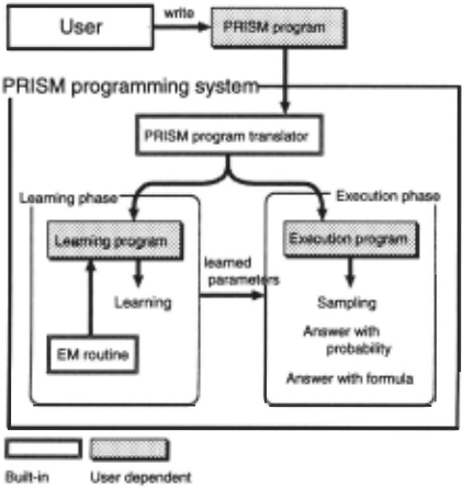
PRISM programming goes through three phases: pro gramming, learning and execution. Since the learning phase and the execution phase require rather different treatment of an original program, PRISM translates it into two specialized programs, one for execution and the other for learning. The latter works in the learning phase cooperating with the built-in EM learning routine to per form maximum likelihood estimate.
5.1 Structure of a PRISM Program
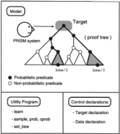
A PRISM program is comprised of three parts, a model, a utility program and the control declarations (Figure 2). The model part is just a logic program whose purpose is to generate possible proof trees of a target atom which represents our observations. Those trees may or may not contain special built-in predicate bsw/3. Since bsw/3 is probabilistic, so can be the target atom, and the problem is to make the distribution of the target atom as close to the observed (empirical) distribution as possible. This is achieved in the learning phase by tuning the parameters of bsw/3 atoms.
The utility part contains a logic program that makes use of the distribution PvB with special built-ins such as learn/0-1 for learning and prob/1-2 and cprob/2-3 for calculation of probabilities. The model part and the utility part should be conceptually distinguished, but actually, when combined, they look like just a logic pro gram with special built-ins.
The control declarations give information required for the learning phase. Currently, we have target declara tion for specifying a target atom, and data declaration for specifying a file containing teacher data (randomly sampled target atoms).
5.2 Learning phase
The learning phase starts with commands learn/0-1. Prior to them, we have to specify a target atom by target declaration, and the data file by data declaration.
Teacher data are expressed as ground literals contain ing the target atom. They are henceforth called goals. What PRISM does in the learning phase is to adjust sta tistical parameters (associated with bsw/3) to maximize the conjunctive probability of these goals. Presently for practical reasons, only positive goals are allowed as teacher data.
PRISM, given the goals in the data file, builds a ta ble to keep the records of the correspondence between a goal and the conjunctions of bsw/3 atoms that ap pear in one of the proof trees of the goal. It means that PRISM computes all solutions, by top-down exhaustive search, and hence sometimes becomes computationally inefficient compared to specialized algorithms developed for specific tasks. Anyway, after completing the table, PRISM sets random values (between 0 and 1) to sta tistical parameters associated with bsw/3 atoms in the table. The EM learning routine then starts to update these parameters iteratively until convergence to attain the maximum likelihood estimators.
5.3 Execution phase
After learning, we run the learned program to check how it learned or how it behaves. There are three execution modes, i.e. sampling, answer with probability and answer with formula.
A special command is used to specify the execution mode. Sampling is done by the command sample/1. For example, for query I ?- sample (bloodtype (X)) the system returns the answer X=a, X=b, X=o or X=ab according to the distribution of bloodtype/1. The commands prob/2 and cprob/3 are used for the answer with probability mode; for the query I ? prob(bloodtype(a) ,Prob) we have Prob=0.4 for in stance. In the case that the given formula is false with probability 1 such as bloodtype (a) & bloodtype (b) we have answer no.
The commands probf/1 and probf/2 give answers with formula. The formula is a DNF of bsw/3 atoms which logically explains the given formula. For example, the answer with formula for bloodtype (a) is
bsw(1, father, 1) 1\ bsw(1 ,mother, 1) V bsw(1,father,1) 1\ bsw(1,mother,1) 1\ bsw(2,mother,O) v6 Examples
In this section, we present modeling examples by PRISM programs, together with learning results.
6.1 Blood type
The first one is the blood type program in Section 3. In case of Japan, the ratio of blood types is A:O:B:AB = 4:3:2:1. We artificially generated random data with this ratio and used them as teacher data for the pro gram to estimate the probability distribution of gene/2. The result is shown in Table 1. Conv shows converged parameters values of the bsw/3 named ID.
| ID | Conv | gene(P,a) | 0.292 |
| 1 | 0.292 | gene(P,b) | 0.163 |
| 2 | 0.230 | gene(P,o) | 0.545 |
| bloodtype(a) | bloodtype(o) |
| bloodtype(b) | bloodtype(ab) |
6.2 HMM
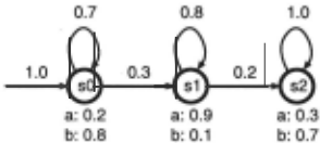
The hidden Markov model (HMM) [Rabiner 89], which has long been a basic tool for speech recognition, stands for a class of finite state automata in which transition is probabilistic and an alphabet is emitted on each transi tion. What we can observe from outside is only an out put string consisting of emitted alphabets while the state transition is not observable, hence the name of HMM. Figure 3 is an example of HMM that has a state set {sO, s1, s2} and output alphabets {a,b}. We can see from the figure that the transition probability from sO to sO is 0. 7 whereas that of sO to s1 is 0. 3. We can also see that on a transition from sO, a is emitted with probability 0. 2 and b with probability 0. 8 etc.
This HMM is described by a PRISM program on next page (the utility part is not shown). For learning, we limit the length of output strings to 5 and leave all pa rameters associated with bsw/3 undefined.
A learning experiment was conducted using 500 teacher data 4 generated from the HMM in Figure 3. We then let the program learn the data placed on the file hmm. dat by the PRISM's built-in EM learning routine. Convergence is judged when an increment of the loga rithmic likelihood of the conjunction of all hmm/1 atoms (teacher data) becomes less than 10- 6 . The result is shown in Table 2 (Smp shows original parameter values).
In PRISM, the probabilities of atoms are com puted by prob/2 predicate and the probability of prob(hmm([a,a,b,a,b]) ,P) is
?- prob(hmm([a,a,b,a,b]),P).
p = 0.05477 ?
This experiment exemplifies the expressive power of PRISM and the learnability of HMMs. It is however
4 These data were obtained from running the HMM pro gram in sampling mode.
-------------HMM program % Initial state is sO with probability 1hmm(L) :- init(S),hmm(1,S,L). % Terminate at T=5 hmm(5, S, [Obs]) :- output (5, S, Obs) . hmm(T,S, [ObsiL]) :- T<5, % Output Obs in state S at time T output(T,S,Obs), % Transit from S to Next at time T trans(T,S,Next), T1 is T+1, hmm(T1,Next,L) . init(sO). %Transition probability pamameters : trans(T,s0,s1) bsw(1,T,1) . trans(T,sO,sO) bsw(1,T,O) . trans(T,s1,s2) bsw(2,T ,1) . trans(T,s1,s1) bsw(2,T,O). trans(_,s2,s2). % Output probability parameters: output(T,sO,a) bsw(3,T,1) . output(T,sO,b) bsw(3,T,O) . output(T,s1,a) bsw(4,T,1) . output(T,s1,b) bsw(4,T,O) . output(T,s2,a) bsw(5,T,1) . output(T,s2,b) bsw(5,T,O) . target(hmm,1) . data('hmm.dat').not sufficient to claim practical usability of PRISM, because the practical merit of using HMMs resides in the availability of three efficient algorithms for three basic problems. Namely, the forward-backward algo rithm [Rabiner 89] for calculating the probability of a given string, the Viterbi algorithm [Rabiner 89] for de ciding the most likely state transition sequence for the given string and · the Baum-Welch learning algorithm (Rabiner 89] to estimate the probability parameters of an HMM. We expect that since PRISM is a general pro gramming language, it will not be very difficult to write PRISM programs for these algorithms.
| ID | Smp | Conv |
|---|---|---|
| 1 | 0.60 | 0.574 |
| 2 | 0.30 | 0.319 |
| 3 | 0.70 | 0.672 |
| 4 | 0.20 | 0.198 |
| 5 | 0.85 | 0.849 |
6.3 Bayesian networks
Now we turn to Bayesian networks [Pearl 88]. Bayesian networks are a knowledge representation language to represent statistical dependencies among random vari ables. We confine ourselves to a case where random variables are binary, i.e. propositions. Dependencies are expressed as a directed acyclic graph where nodes repre sent propositions and links indicate direct probabilistic dependencies quantified with probabilities. The graph as a whole represents a joint probability distribution of propositions. For example 5 , In Figure 4, it holds that
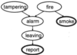
P( Tamering, Fire, Alarm, Smoke, Learving, Report) = P(Report I Leaving)P(Leaving I Alarm) P(Alarm I Tampering, Fire )P(Smoke I Fire) P( Fire) P( Tampering)Following [Poole 93), we describe this Bayesian net work as follows: Bayesian network program l target(world,6) . data('world.dat'). % Joint distribution: world(Ta,Fi,Al,Sm,Le,Re) fire(Fi),tampering(Ta),c_smoke(Sm,Fi), c_alarm(Al,Fi,Ta),c_leaving(Le,Al), c_report(Re,Le) . smoke(Sm) :- fire(Fi),c_smoke(Sm,Fi). alarm(Al) : fire(Fi),tampering(Ta),c_alarm(Al,Fi,Ta) . leaving(Le) :- alarm(Al),c_leaving(Le,Al) . report(Re) :- leaving(Le),c_report(Re,Le) . tampering(yes) : - bsw(ta,none,1) . tampering(no) :- bsw(ta,none,O). fire(yes):- bsw(fi,none,1). fire(no) :- bsw(fi,none,O) . c_smoke(yes,Fi):- bsw(sm(Fi),none,1) . c_smoke(no,Fi) :- bsw(sm(Fi),none,O) . c_alarm(yes,Fi,Ta):- bsw(al(Fi,Ta),none,1). c_alarm(no,Fi,Ta) : - bsw(al(Fi,Ta),none,O) . c_leaving(yes,Al):- bsw(le(Al),none,1). c_leaving(no,Al) :- bsw(le(Al),none,O) . c_report(yes,Le):- bsw(re(Le),none,1). c_report(no,Le) :- bsw(re(Le),none,O) .5 This example is taken from [Poole 93).
| ID | Smp | Conv | ID | Smp | Conv |
|---|---|---|---|---|---|
| fi | 0.10 | 0.116 | ta | 0.15 | 0.160 |
| sm(yes) | 0.95 | 0.966 | sm(no) | 0.05 | 0.054 |
| al(yes,yes) | 0.50 | 0.250 | al(yes,no) | 0.90 | 0.880 |
| al(no,yes) | 0.85 | 0.889 | al(no,no) | 0.05 | 0.049 |
| le(yes) | 0.88 | 0.898 | le(no) | 0.01 | 0.016 |
| re(yes) | 0.75 | 0.769 | re(no) | 0.10 | 0.082 |
An experiment was conducted using 500 teacher data sampled from the above program with parameter values shown as Smp in Table 3. Convergence is obtained after two iterations of the EM learning routine and the con verged parameter values are shown as Conv in Table 3.
After learning, we can check various probabilities by using built-in predicates such as prob/2 and cprob/3. For instance, P( Fire I Smoke, ·Alarm), the probability of a fire breaking out while smoke is observed but the alarm is not ringing, is
I ?- cprob(fire(yes),(smoke(yes),alarm(no)),P).
p = 0 . 27739 ?7 Related work
PRJSM is a general programming language with the abil ity of learning, and we don't have many predecessors with the same character and power. Probably, most di- · rectly related one is Poole's Probabilistic Horn abduction [Poole 93). His semantics however excludes large part of usual logic programs 6 . Furthermore probabilities are considered only for finite cases (no joint distribution for infinitely many random variables). Accordingly there is no way to express Markov chains such as HMMs.
Ng and Subrahmanian proposed Probabilistic Logic Programming [Ng 92). Their approach is based on in tervals. They assign probability ranges to atoms in the program and check, using linear programming technique, if probabilities satisfying those ranges actually exist or not. The use of linear programming confines their ap proach to a finite domain. Neither of Poole's proposal or Ng and Subrahmanian' proposal mentions learning.
Charniak and Goldman proposed a special lan guage FRAIL3 for construction of Bayesian networks [Charniak et al. 93). Although their rules look much like definite clauses annotated with probability depen dencies, the semantics is not very clear and no learning mechanism is provided for their programs.
Hashida [Hashida 94) proposed a rather general frame work for natural language processing as probabilistic constraint logic programming. He assigned probabilities to between literals and let them denote the degree of the probability of invocation. He has shown constraints are efficiently solvable by making use of these probabilities.
6 This is due mainly to the acyclicity assumption made in [Poole 93] .
8 Conclusion
We have presented PRJSM which is a new modeling lan guage for symbolic-statistical phenomena. It not only has general computing power combined with probabilis tic semantics but also has a general learning mechanism that enables any PRISM program to learn from exam ples. Below are two potential application areas.
PRJSM programs can define Markov chains such as HMMs with mathematical rigor. Using this property, and taking advantage of PRISM's first order expressive ness, it looks feasible to describe Markov decision pro cesses controlled by complex symbolic reasoning. This might contribute to modeling agents with rich knowl edge, interacting and learning one another.
NLP is another promising area because of the obvi ous need for describing statistical correlations between syntactic structures and semantic structures. It is also noticeable that a large corpus is already available for learning.
Computation power and learning power should be unified to give a new dimension to programming. We hope that PRJSM brings us one step closer to the cross fertilization of computation and learning.
@inproceedings{ijcai1997p192,
  title     = {PRISM: A Language for Symbolic-Statistical Modeling},
  author    = {Sato, Taisuke and Kameya, Yoshitaka},
  booktitle = {Proceedings of the Fifteenth International Joint Conference on
               Artificial Intelligence, {IJCAI-97}},
  publisher = {International Joint Conferences on Artificial Intelligence},
  editor    = {Martha E. Pollack},
  pages     = {1330--1338},
  year      = {1997},
  note      = {Probabilistic Reasoning},
  url       = {https://ijcai.org/proceedings/1997/192},
}
TY - CPAPER TI - PRISM: A Language for Symbolic-Statistical Modeling AU - Sato, Taisuke AU - Kameya, Yoshitaka T2 - Proceedings of the Fifteenth International Joint Conference on Artificial Intelligence, IJCAI-97 PB - International Joint Conferences on Artificial Intelligence PY - 1997 SP - 1330 EP - 1338 UR - https://ijcai.org/proceedings/1997/192 ER -Copied
Machine-readable versions of this paper, for tools and AI agents:





