Space-Efficient Inference in Dynamic Probabilistic Networks

1 Introduction

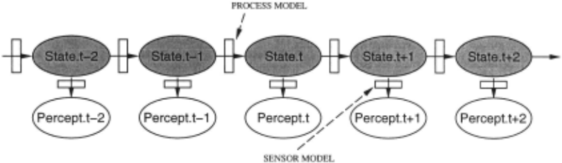
Dynamic probabilistic networks are variants of prob­ abilistic (Bayesian) networks designed to represent stochastic temporal processes. They were first used ex­ tensively by Dean and Kanazawa [1989], and have since become a standard tool in AI. As Figure 1 shows, a DPN consists of infinitely repeated slices; the variables in the t 'th slice represent the state of the process at time t . We assume for the sake of expository simplicity that the variables within a slice can be divided into state variables Xt : which are always hidden, and evidence variables Et , wh1ch are always observable. We also assume that only adjacent time slices are connected, and that the topolog­ ical structure and conditional distributions are identical for all time slices. That is, the DPN is specified by defin­ ing the structure and interconnectivity of the first two slices, and this is then "unrolled" N times, to provide storage space to hold the Xt and Et values fort E (0 , N] .

If there is only one hidden variable and one observ­ able variable per time slice, a DPN is equivalent to a Hidden Markov Model (HMM). The main advantage of DPNs over HMMs arises when the state can be decom­ posed into several state variables, as in Figure 2. (Thus, Ghahramani and Jordan [1995] refer to DPNs as "facto­ rial HMMs ." ) If each state variable is directly influenced by at most a constant number of other variables, then the number of parameters required to specify the DPN will be linear in the number of state variables, whereas for standard HMMs it is exponential. This reduction makes both inference and learning potentially much more effi­ cient.

This paper begins with a discussion of the DPN mon­ itoring task-that is, computing a posterior distribution for the state variables at each time step given all obser­ vations up to that time. Recursive, constant-space algo­ rithms are well-known for monitoring in DPNs and other models . We then discuss the problem of hindsight- that is, computing a posterior distribution given both past and future observations. Hindsight is an essential sub­ task of learning DPN models from data. Existing al­ gorithms for hindsight - which simply unroll the DPN and treat it like a static network - use O(SN) space and time, where N is the total length of the observation sequence and S is the state space size for each time step.

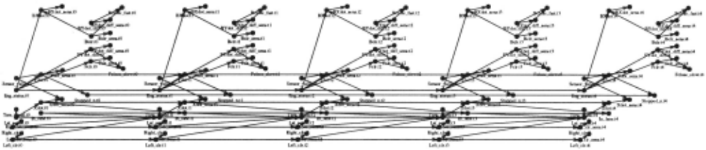
They are therefore impractical for hindsight in complex models with long observation sequences. As an example of the severity of the space problem, we note that the net­ work in Figure 2 has S ~ 10 6 and, during model learn­ ing, may require N ~ 10 5 . Therefore, we present a sim­ ple divide-and-conquer algorithm that reduces the space requirements from O(SN) to O(SlogN), thus making such applications feasible in practice. We present exper­ imentals results to validate our .claims. We also briefly discuss a possible way of reducing the space requirements even more dramatically, namely to use only O(S) space. This would be particularly useful for online learning al­ gorithms.

2 Monitoring in DPNs

The most common use of DPNs is for monitoring, i.e., computing P(XtiEo:t), where we use the notation E;:j as shorthand for the variables E;, ... , Ej. In this capacity, a DPN allows one to keep track of the state of a process given partial, noisy observations. For example, one could estimate the progress of a disease in a patient from clin­ ical observations over time, or estimate the position of a missile from a sequence of radar observations. In con­ trol theory, this task is called filtering. The well-known Kalman filter [Kalman, 1960] can be viewed as a special case of a continuous-variable DPN in which the sensor model is restricted to be Gaussian and the process model is restricted to be linear with Gaussian noise [Alag and Agogino, 1996]. We note that DPNs can handle a much larger variety of processes than Kalman filters.

Standard arguments (see e.g., [Russell and Norvig, 1995, p.509]) show that monitoring corresponds to the following recursive update equation

where a is a normalizing constant. For future reference, we represent this equation more abstractly as

where we have introduced the forward probabilities Ft = P (Xt I Eo t) . We assume the initial "boundary condition" Fa is known.

The process of computing the forward probabilities can be implemented in a variety of ways. Kjaerulff [1992] describes dHugin, an extension of the Hugin package that handles DPNs via direct manipulation of the join tree. Russell and Norvig [1995] describe the roll-up method , which operates directly on the DPN. Finally, one can implement Equation 1 simply by enumerating over the possible states Xt.

The space and time complexity of monitoring can be expressed in terms of N, the total number of time steps; lEI, the number of evidence variables per time step; lXI, the number of state variables per time step; and S, the space required to store the probability distribution over X 1 . In the worst case, S = 2IXI, which corresponds to a completely connected network, even if the original DPN was only sparsely connected. This is because condition­ ing on past evidence causes variables in the current slice to become directly dependent. 1 Storing all the input (Et for all t) and output (F1 for all t) takes O(NIE\) and O(N S) space respectively. However, it is reasonable to assume that the input is available as a stream from the environment or is read in sequentially from secondary storage, and similarly for the output. That is, we assume that there are "producer" and "consumer" processes for the input and output; we just focus on the amount of temporary working space required by the montoring al­ gorithm itself, namely O(S). The time required is of course O(SN).

The related task of prediction, computing P(Xt lEoN) for t > N, can be performed by running a monitoring algorithm with no evidence beyond N, and hence also requires O(S) working space.

3 Hindsight in DPNs

In some settings, we may wish to take "future" evidence, as well as past and present evidence, into account e.g., where the t index does not refer to time, but is simply an index into a static sequence. The observations after t may help to eliminate uncertainty about the state at t. For example, one can deduce who was in the house at the time of the murder by subsequent observation to see who leaves the house, even if one neglected to observe the house prior to the murder. The process of comput­ ing P(Xt IEo:N) for t E (0 . . . N] is called smoothing in control theory, where it is often used to reduce the ap­ parent wiggliness in a trajectory computed by filtering. In AI, perhaps the most important use of hindsight is in learning. In order to learn a DPN model from observa­ tion sequences, it is necessary to compute likelihoods for the hidden variables given all available data [Lauritzen, 1995; Russell et al., 1995], hence hindsight is an integral part of DPN learning.

The most obvious algorithm for hindsight is to perform monitoring in the forwards and backwards directions, and to combine the information at each time step, as follows:

where we have introduced the combination operator and the quantity B1 = P(Et+l:N IXt) to denote the back­ wards probabilities. These can be updated as follows:

1 Technically, the joint distribution has only the indepen­ dences present in the stationary distribution of the Markov chain represented by the DPN.

BackOp(Bt+l, Et+d

Again, we assume the boundary condition BN is known. We can think of this method as propagating the for­ wards and backwards "messages" Ft and Bt from both ends towards slice t (which takes O(SN) time and 0(5) working space), combining them, and then repeating for each t. Hindsight for the complete sequence therefore requires O(N 2 S) time and O(S) working space.

By storing F t and Bt at each time step (i.e., caching intermediate results), we get an algorithm that is es­ sentially identical to Pearl's rr->. message-passing algo­ rithm for chains, to the join-tree algorithm operating on an explicitly represented DPN with N slices , or to the forward-backward HMM algorithm (see also [Smyth et al., 1996]). All these approaches require O(SN) time, but unfortunately require O(SN) space, which is im­ practical. We now go on to discuss a simple divide-and­ conquer algorithm that requires O(SN log N) time and O(S log N) space.

4 The space-efficient algorithm

The essential idea of our space-efficient method is to store the F t and Bt messages at k - 1 intermediate "checkpoints" or "islands", thereby dividing the origi­ nal sequence into k segments; we then recursively ap­ ply the hindsight algorithm to each smaller segment , making use of the boundary conditions stored at each checkpoint. For example, if N = 24 and k = 2, we compute F 1 , F2, ... , F24 and B23, B22 , ... , Bo by itera­ tively applying the forward and backward operators to the boundary conditions Fa and B24 respectively, but we only store F1 and B1 for t = 12. We compute P(XdEoN) = CombineOp(F12, B12), pass it to the consumer 2 , and then recursively apply the hindsight al­ gorithm to the sub-sequences for t = 1 . . . 11, using Fa and B12 as boundary conditions, and for t = 13 ... 23, using F 12 and B24 as boundary conditions.

The total working space required by this approach is determined by two parameters: k, the number of check­ points we store at each level, and D, the number of lev­ els of recursion before we invoke the base case algorithm (which uses linear time and linear space). If we treat k as a fixed parameter, and recurse "all the way to the bot­ tom" (i.e., apply the base case only to segments of length 1), we have D = logk N. The working space is then O(kSlogk N), since we store k checkpoints, each of size 25, at each level of recursion, and there are D = logk N levels of recursion. The time required by this approach, T( N), is the time taken to propogate the messages ac~oss k segements of length roughly N / k each, plus the t1me to solve the k subproblems: T(N) = k(N/k) +kT(N/k) , so T(N) = N logk N. We can decrease the running time, and increase the space requirements, either by increas­ ing k from 2 to N, or by decreasing D from logk N to 1.

2 The consumer might store P(X12IEo:N) on secondary storage, or it might use it in a learning algorithm to perform an in-place update of the model parameters, before discard­ ing it .

An interesting compromise is k = VN, which takes only twice as long as the standard algorithm and needs only O(SVN) space.

5 Experimental results

We have implemented the abstract operators FwdOp, BackOp, and CombineOp in terms of a modified version of the Jensen join tree algorithm [Jensen et al., 1990]. The details will be presented in another paper, but the basic idea is to modify the triangulation heuristic to en­ sure that the resulting join tree has a repeating structure. This repeating block may span two slices in the original network (i.e., it might contain cliques which have nodes from adjacent slices), so that Ft and Bt now refer to the forwards and backwards messages associated with the t'th repetition of this block, rather than the t'th time slice.

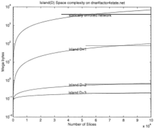
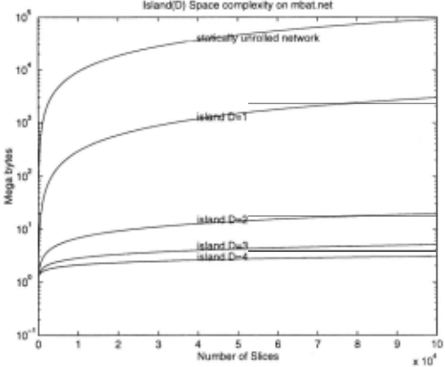
In Figure 4, we show how much space is required to do inference on the simple network shown in Figure 3 as a function of the length of the sequence. It is clear that by increasing the depth of recursion, D, we can reduce the space requirements dramatically. The time taken for D = 1 with N = 100 was 1.5 seconds , for D = 2 it was 1.96 seconds, and for D = 3 it was 2.6 seconds. 3 In Figure 5, we plot a similar curve for the more complicated network shown in Figure 2.

6 Further work: Constant space?

We have shown how to avoid the otherwise crippling space requirements for hindsight in DPNs, giving an al­ gorithm whose space complexity grows logarithmically with the length of the sequence. This has allowed us to address far more complex DPN learning problems than previously possible.

An analogous technique could be applied to cope with cases where S (and not just N) is very large. The idea would be to store check points for only some of the nodes within a slice. For example, in the join tree algorithm, instead of storing messages at every node in the repeat­ ing tree structure, we could store messages at only some of them, recomputing the others on demand . 4 This could of course be combined with the current approach to yield an O(log N log S)-space algorithm.

A more ambitious goal would be to find a constant­ space algorithm, that is, one having space requirements which are independent of N. This would be particu­ larly useful in the context of online learning, in which a continuous stream of evidence is arriving (and hence N grows indefinitely) . We currently only know how to do this in restricted circumstances. The idea is as follows. According to Equation 4, we can compute the posterior at time step t given Ft and Bt. We can filter forward all the way to the end to obtain F N, and B N is given. By backward monitoring, we can now compute BN_1 . If we can also compute FN_1 from FN, we are in business. This can be done by inverting the process model and by undoing the effects of EN . We then continue this pro­ cess all the way back to the beginning of the sequence, computing posteriors as we go.

3 Experiments were run on a Pentium Pro 200MHz PC with 64 Megabytes of RAM, using Linux and gee.

4 The key requirement is that the set of nodes at which we choose to store checkpoint information d-separate the evidence.

The details of the inversion process are best under­ stood in terms of matrix operations , where we consider F t as a vector of probabilities over all possible states Xt of the variables in Xt . Let Ot be the diagonal ma­ trix whose entries are the probabilities in P(EtiXt), and let M, the transition matrix, contain the probabilities P(Xt+1/Xt) for all values Xt+1 and Xt. (Note that ac­ cording to our assumptions, M is independent of time.) Equation 1 now becomes the vector equation

From this we can obtain the inverse operation:

Thus, in the generic case where M and 0 are invertible, we have a constant-space hindsight algorithm. This al­ gorithm will fail, however, if either matrix is singular. Ot will be singular only if some entries in P(EtiXt) are zero, that is, if the observations rule o-ut some of the possible states. M will be singular if, for example, two columns are identical- which could easily occur if transi­ tions are independent of one of the state variables. Thus, invertibility will fail in many realistic situations where information is lost as the process proceeds, and in many others the inversion step will be highly ill-conditioned. It remains to be seen whether it is possible to somehow store a small amount (independent of N) of extra infor­ mation to make the transformation invertible.

Acknowledgments

Thanks to Paul Horton, Geoff Zweig, Nir Friedman, and the reviewers for useful comments.