
Avoiding Overfitting with BP-SOM
Proceedings of the Fifteenth International Joint Conference on Artificial Intelligence. Neural Networks. Pages 1140-1144.
© 1997 International Joint Conferences on Artificial Intelligence
Abstract
Overfitting is a well-known problem in the fields of symbolic and connectionist machine l ea rning. It describes the deterioration of generalisation performance of a trained model. In this paper , we investigate the ability of a novel artificial neural network , BP -S OM , to avoid overfitting. BP-SOM is a hybrid neural network which combines a multi-layered feed-forwa rd network (MFN) with Kohon en 's self-organising maps (soMs). During training, supervised back-propagation learning and unsupervised SOM learning cooperate in finding adequate hidden-layer representations . We show that BP-SOM outperforms standard backpropagation, and also back-propagation with a weight decay when dealing with the problem of overfitting. In addition, we show that BP-SOM succeeds in preserving generalisation performance under hidden-unit pruning , where both other m et hods fail.
- [Cun et al., 1990] Y. Le Cun, J. Denker, and S. Solla. Optimal brain damage. In D . S. Touretzky, editor, Advances in Neural Information Processing Systems, volume 2, pages 598-605.
- Morgan Kaufmann, San Ma- teo, CA, 1990.
- [Fahlman and Lebiere, 1990] S. E. Fahlman and C. Lebiere . The cascade-correlation learning archi- tecture. Technical Report CMU-CS-90-100, School of Computer Science, Carnegie-Mellon University, Pitts- burgh, PA, 1990.
- [Hassibi et al., 1992] B. Hassibi, D. G. Stork, and G. J. Wolff. Optimal brain surgeon and general network pruning. Technical Report CRC-TR-9235, RICOH California Research Centre, 1992.
- [Hinton, 1986] G. E. Hinton. Learning distributed rep- resentation of concepts. In Proceedings of the Eighth Annual Conference of the Cognitive Science Society, pages 1-12, Hillsdale, NJ, 1986. Erlbaum.
- [Jordan and Bishop, 1996] M. I. Jordan and C. M. Bishop. Neural networks. Technical Report A.l. Memo No. 1562, Artificial Intelligence Laboratory, Massachusetts Institute of Technology, 1996.
- [Kohonen, 1984] T. Kohonen. Self-organisation and As- sociative Memory, volume 8 of Series in Information Sciences. Springer-Verlag, Berlin, 1984.
- [Mozer and Smolensky, 1989] M. C. Mozer and P. Smolensky. Using relevance to reduce network size automatically. Connection Science, 1:3-16, 1989.
- [Norris, 1989] D. Norris. How to build a connectionist idiot (savant). Cognition, 35 :277-291, 1989.
- [Prechelt, 1994] L. Prechelt. Probenl: A set of neu- ral network benchmark problems and benchmarking rules. Technical Report 19/94, Fakultiit fiir lnfor- matik, Universitiit Karlsruhe, Germany, 1994.
- [Quinlan, 1993] J . R . Quinlan. c 4 .5: Programs forMa- chine Learning.
- Morgan Kaufmann, San Mateo, CA , 1993.
- [Rissanen, 1983] J. Rissanen. A universal prior for inte- gers and estimation by minimum description length. Annals of Statistics, 11:416-431, 1983.
- [Rumelhart et al., 1986] D . E. Rumelhart, G . E. Hinton, and R . J. Williams. Learning internal representations by error propagation. In D. E. Rumelhart and J . L. McClelland, editors, Parallel Distributed Processing: Explorations in the Microstructure of Cognition, vol- ume 1: Foundations, pages 318-362. The MIT Press, Cambridge, MA, 1986.
- [Shaffer, 1993] C . Shaffer. Overfitting avoidance as bias. Machine Learning, 10:153-178,1993.
- [Thornton, 1995] C. Thornton. Measuring the difficulty of specific learning problems. Connection Science , 7:81-92, 1995.
- [Weigend et al., 1990] A. S. Weigend, D. E. Rumelhart, and B. A. Huberman. Generalization by weight- elimination with application to forecasting. In R. P. Lippman, J. E. Moody, and D . S. Touretzky, editors , Advances in Neural Information Processing Systems, volume 3, pages 875-882 .
- Morgan Kaufmann, San Ma- teo, CA, 1990.
- [Weigend, 1994] A. S. Weigend. On overfitting and the effective number of hidden units . In M. C. Mozer, P. Smolensky, D. S. Touretzky, J. L. Elman, and A. S. Weigend, editors, Proceedings of the 1993 Connection- ist Models Summer School, pages 335-342, 1994.
- [Weijters, 1995] A. Weijters. The BP-SOM architecture and learning rule. Neural Processing Letters, 2:13-16, 1995. .
- [Wolpert, 1992] D. H. Wolpert. On overfitting avoidance as bias. Technical Report SFI TR 92-03-5001, The Santa Fe Institute, 1992.
References were extracted automatically from the PDF and may contain errors.
Full text extracted automatically from the PDF; figures, tables and equations may differ. The PDF is the version of record.
1 On avoiding overfitting
In machine-learning research, the performance of a trained model is often expressed in its generalisation per formance , i.e., its capability to process correctly new in stances not present in the training set. When the gener alisation performance of the trained model is much worse than its performance on the training material (i.e., its ability to reproduce the training material), we speak of overfitting. Overfitting is sometimes due to the sparse ness of the training material: e.g., the training material does not sufficiently cover the characteristics of the clas sification task. A second cause for overfitting might be a high degree of non-linearity in the training material. In both cases, the learning algorithm might not be able to learn more from the training material than the classi fication of the training instances itself (see, e.g., Norris , 1989).
The issue of avoiding overfitting is well-known in the field of symbolic and connectionist machine learning (e.g., Wolpert, 1992; Schaffer, 1993; Jordan and Bishop, 1996) . In symbolic machine learning, a commonly used heuristic to avoid overfitting is rmmrmsmg the size of the induced models (cf. Quinlan's (1993) C4.5 and C4.5rules), in the sense of the minimum-description length (MDL) principle (Rissanen, 1983). For instance, smaller (or less complex) models should restrict the num ber of parameters to the minimum required for learning the task at hand.
In connectionist machine learning (neural networks) , avoiding overfitting is closely related to finding an op timal network complexity. In this view, two types of methods of avoiding overfitting (or regularisation) can be distinguished: (i) starting with an undersized net work and gradually increasing the network's complexity (Fahlman and Lebiere, 1990), and (ii) starting with an oversized network and gradually decreasing its complex ity (e.g., Mozer and Smolensky, 1989; Le Cun, Denker, and Solla, 1990; Weigend, Rumelhart, and Huberman, 1991; Hassibi, Stork, and Wolff, 1992; Prechelt, 1994; Weigend, 1994) .
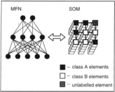
In this paper we analyse the overfitting-avoidance be haviour of a novel artificial neural-network architecture (BP-SOM, Weijters, 1995) , which belongs to the sec ond type of connectionist machine-learning methods. In BP-SOM, the network complexity is reduced by guiding the hidden-layer representations of a multi-layer feed forward network (MFN, Rumelhart et al., 1986) to sim plified vector representations. To achieve its aim, BP SOM combines the traditional MFN architecture with self organising maps (soMs) (Kohonen, 1984): each hidden layer of the MFN is associated with one SOM (see Fig ure 1) . During training of the weights in the MFN, the corresponding SOM is trained on the hidden-unit acti vation patterns. The standard MFN error~signal is aug mented with information from the SOMs. The effect of the augmented error signals is that , during learning, the hidden-unit activation patterns of clusters of instances associated with the same class tend to become highly similar. Intuitively speaking, the self-organisation of the SOM guides the MFN into arriving at adequate hidden unit representations.
We demonstrate that BP-SOM avoids overfitting by re ducing the complexity of the hidden-layer representa tions. In Section 2, we provide a description of the BP-SOM architecture and learning algorithm. Section
3 presents experiments with BP-SOM trained on three benchmark classification tasks, focusing on the ability to avoid overfitting. In addition, we study the robust ness of BP-SOM to hidden-unit pruning. Our conclusions are given in Section 4.
2 BP-SOM
Learning in BP-SOM is a cooperation between supervised learning in BP and unsupervised learning in SOM. The unsupervised dimension reduction and clustering on the SOM guide BP learning during the development of ad equate hidden-layer representations on the MFN. The influence of the SOM causes clusters of hidden-layer rep resentations associated with the same class, to become increasingly similar to each other. In this section we describe how the cooperation between BP and SOM is implemented.
2.1 The BP-SOM architecture
The BP-SOM architecture is composed of two types of well-known building blocks, viz. an MFN combined with one or more SO Ms. The number of SOMs equals the num ber of hidden layers in the MFN; each SOM is associated with one hidden layer. Figure 1 illustrates a BP-SOM network with five input units, one hidden layer with four units, two output units, and one SOM. The size of the SOM is arbitrarily chosen to be 3 x 3. Each of the nine elements, denoted by Ei ( i = 1, ... , 9), contains an acti vation vector, denoted by VE;, of length 4 (equal to the number of hidden units), a class label, two class counters (equal to the number of output classes), and a reliability value field.
2.2 The BP-SOM learning algorithm
We assume that BP-SOM, with l hidden layers and l as sociated SOMs (l ~ 1), is trained on a classification task with two or more distinct output classes . Training of the MFN and SOMs proceeds in parallel as follows : after feed-forward activation of an input instance, vhidden' the activations of the units of each hidden layer of the MFN
part are used as learning vectors for the corresponding SOM. Each SOM is trained with Kohonen's (1989) SOM learning algorithm. After a number of training cycles (epochs), each SOM starts to develop topological order. Each SOM element is assigned an output-class label. The procedure for determining these labels is as follows: af ter each nth training cycle, all training instances (with known output classes) are presented one by one to the MFN. Each instance generates a pattern Vhidden on the hidden layer. The winning SOM unit Ei is the unit whose VE; has the smallest Euclidean distance to vhidden. For each instance, the appropriate class counter of the win ning unit is incremented by one. After all instances have been presented, the largest class counter of each unit defines its label. For example, let the BP-SOM network displayed in Figure 1 be trained on a task which maps instances to either output class A or B. If a SOM ele ment Ei is the best matching element to 4 activation vectors that map to class A, and to 2 activation vectors that map to class B, the class label of Ei is 'A', with a reliability of 4/6 = 0.67. This value is assigned to the reliability value field of Ei . As a result, we can visually distinguish areas in the SOM: areas containing elements labelled with class A and class B, and areas containing unlabelled elements (no winning training instances could be found). In Figure 1, we see four class labels A, four class labels B, and one element unlabelled.
For each training instance, the BP part of BP-S OM gen erates an error vector, Vbp_error, for the hidden units . In BP-SOM the complexity of the MFN is constrained by augmenting Vbp_error with the class information of the corresponding SOM. The BP-SOM algorithm searches for the winning element Ei of those elements that are la belled with the same output class associated with the instance. It should be noted that this SOM element Ei may not be the overall best-matching element, since there may be another element labelled with an output class different from vhidden that matches vhidden better. In other words, the best-matching element labelled with the same Class is searched for, and not the overall best matching SOM element. Taking the difference between the vectors VE; and Vhidden results in a SOM error vector V,om_error. If there is no SOM element labelled with the output class of vhidden' all elements of V.om_error are set to zero. The error vector of a hidden unit j, referred to as Vbp_.om_errori is defined as
Here a denotes the influence of V.om_error on the learn ing process (in our experiments, a is typically set to 0.25 ; a = 0 corresponds to standard BP). The parameter a determines the degree to which the vhidden is trained to be more similar to VE;. The parameter r denotes the reliability of the winning SOM element Ei as described above; tis a threshold parameter, typically set to 0.95.
- Initialise the MFN and the corresponding SOMs (i.e., as sign random numbers within predefined bounds to all connection weights and SOM-element vectors). Initialise the class labels, the class counters, and the reliability field of all SOM elements to unlabelled, zero, and zero, respectively.
- Train the MFN during a fixed number of cycles ( m ). For each cycle do
- For each training instance with its associated output class in the training set:
- Compute the MFN output via feed-forward acti vation through the MFN. Collect for all hidden· layers their vhidden, and train the corresponding SOMs on these vectors using Kohonen's (1989) SOM learning algorithm.
- Calculate Vbp_10m-···o· and update the MFN weights according to equation ( 1 ).
- After each nth training cycle ( 1 ~ n ~ m ), re compute the class labels and reliability of all SOM elements by performing a class-labelling procedure as described in the text.
Figure 2: A conceptual description of the BP-SOM learn ing algorithm.
The threshold parameter is used to prevent unreliable SOM elements to influence Vbp-·om-···or. During the last step of processing a training instance, the BP-SOM algo rithm handles the bp_som_error; of each hidden unit in the same way as BP uses the bp_error; in the traditional on-line back-propagation weight-updating rule. A con ceptual description of the BP-SOM learning algorithm is given in Figure 2.
Upon completion of learning, the SOMs become redun dant, as they do not interact with the propagation of activation through the MFN network.
3 Experiments with BP-SOM
In this section, we present three experiments with the BP-SOM architecture and the BP-SOM learning algorithm. In these experiments, we compare BP-SOM with (i) stan dard BP (Rumelhart et al., 1986), and (ii) BP augmented with weight decay (Hinton, 1986), henceforth denoted by BPWD. Weight decay is included in the comparison, as it is a simple, commonly used method for avoiding overfitting in BP-trained MFNS. BP-SOM, BP, and BPWD are trained on three benchmark classification tasks, viz. the date-calculation task, the parity-12 task, and the task of detecting splices in DNA sequences. The date calculation task and the parity-12 task are hard to learn for many learning algorithms, often leading to overfitting (Norris, 1989; Schaffer, 1993; Thornton, 1995), because the output classification in both tasks depends on the values of all input features. For example, knowing the date and the month and not the year makes it impossi ble to estimate the day of the week with a probability greater than chance. The gene-splice detection task does not have this property.
We have used a fixed set of parameters for all three experiments described. The parameter values for BP (in cluding the number of hidden units for each task) were determined by performing pilot experiments with BP , and taking the values which led to optimal validation performance. Hence, the BP learning rate was set to 0.15 and the momentum to 0.4. BP, BPWD, and BP-SOM were trained for a fixed number of cycles m = 2000. The following parameter values, specific for BP-SOM, gave op timal generalisation performance in a number of pilot ex periments on the date-calculation task. In all SOM·s a de creasing interaction strength from 0.15 to 0.05, and a de creasing neighbourhood-updating context from a square with maximally 25 units to only 1 unit (the winner) was used. The influence of the SOM error vector, a, was set to 0.25, and the reliability threshold t to 0.95 . Class labelling in BP-SOM was performed at each fifth cycle (n = 5). The term a was enabled after the first five cycles. Early stopping, a common method to prevent overfitting, was used in all experiments with BP, BPWD, and BP-SOM: the performance of a trained network was calculated in percentages of incorrectly-processed test in stances at the cycle where the classification error on vali dation material was minimal (Prechelt, 1994). The min imal classification error was always reached well within the limit m.
3.1 Improving generalisation performance First experiment: date calculation
Date calculation is an example of a task which easily leads to overfitting in MFNs trained by BP; hence the trained MFN has a low generalisation performance (Nor ris, 1989). The task is: given a certain date (e.g., March 10, 1975), determine the day of the week it fell on (e.g., Monday). Norris (1989) describes a connectionist model of an idiot-savant date calculator, using an MFN and BP. He concluded that BP was not able to learn this task, unless it was decomposed into three easier subtasks.
In our experiments with BP-SOM, we concentrated on the same interval of dates as Norris, i.e., training and test dates ranged from January 1, 1950 to December 31 , 1999. We generated two training sets, each consisting of 3,653 random selected instances, i.e., one-fifth of all dates. We also generated two corresponding test sets and two validation sets (with 1,000 instances each) of new dates within the same 50-year period. In all our ex periments, the training set, test set, and validation set had empty intersections. The date November 23, 1988 is represented by setting unit 23 in the day field to 1, unit 11 in the month field to 1, and unit 39 of the year field to 1. All other 90 input units are set to zero. The output is represented by 7 units, one for each day of the week. The MFN contained one hidden layer with 12 hidden units for BP (found to result in optimal validation performance), and 25 hidden units for BPWD and BP-SOM. The corre sponding SOM of the BP-SOM network was of size 12 x 12. Two different data sets were generated. On each set, five runs with different random weight initialisations were performed with BP, BPWD, and BP-SOM. The average classification errors on the test material for these thirty experiments are reported in the top row of Table 1.
| BP: % incorrect I | BPWD: %incorrect I | BP-SOM: %incorrect I | ||||
|---|---|---|---|---|---|---|
| Task | Train | Test | Train | Test | Train | Test |
| date calc. | 20.8 ±5.4 | 28.8 ±7.8 | 1.5 ± 0.3 | 8.8 ±1.4 | 2.9 ±2.0 | 3.3 ±1.9 |
| parity-12 | 14.1 ±18.8 | 27.4 ±16.4 | 21.6 ±24.2 | 22.4 ±18.3 | 5.9 ±10.2 | 6.2 ±10.7 |
| gene-1 | 12.0 ±7.6 | 22.0 ±6.0 | 4.5 ±1.2 | 13.6 ±1.2 | 4.0 ±1.1 | 11.9 ±0.6 |
| gene-2 | 8.6 ±7.1 | 18.8 ±5.5 | 4.4 ±1. 7 | 13.1 ±0.9 | 3.4 ±0.7 | 10.3 ±0.5 |
| gene-3 | 9.2 ±5.3 | 20.8 ±4.2 | 4.0 ±0.9 | 14.4 ±1.1 | 3.2 ±1.0 | 12.8 ±0.6 |
From Table 1 it follows that the average classifica tion error of BP is high: on test instances BP obtains a classification error of 28.8%, while the classification er ror of BP on training instances is 20.8%. Compared to the classification error of BP, the classification errors on both training and test material of BPWD and BP-SOM are much lower.
However, BPWD's generalisation performance on the test material is seriously worse than its performance on the training material: this is an indication of overfitting. We note in passing that the results of BPWD contrast with Norris' (1989) claim that BP is unable to learn the date-calculation task when it is not decomposed into sub tasks. The inclusion of weight decay in BP is sufficient for a good approximation of the performance results of Norris' (1989) decomposed network.
The results in Table 1 also show that the performance of BP-SOM on the training material is comparable, albeit very roughly, with that of BPWD; however, the perfor mance of BP-SOM on test material is significantly better than that of BPWD (t(19)=7.39, p<0.001). Consider ing that the performances of BP-SOM on training and test material are in the same range, we conclude that for the date-calculation task, BP-so'M has been able to avoid overfitting.
Second experiment: parity-12
BP, BPWD, and BP-SOM were applied to the parity-12 task, viz. the task to determine whether a bit string of O's and 1 's of length 12 contains an even number of 1 's. The training set contained 1,000 different instances selected at random out of the set of 4,096 possible bit strings. The test set and the validation set contained 100 new instances each. The hidden layer of the MFN in all three algorithms contained 20 hidden units, and the SOM in BP-SOM contained 7 x 7 elements. The algorithms were run with 10 different random weight initialisations. The second row of Table 1 displays the classification errors on training instances and test instances. The results again indicate that BP-SOM performs significantly better than BP and BPWD on test material (t(19)=3.42, p<0.01 and t(19)=2.42, p<0.05, respectively), and that BP-SOM is able to avoid overfitting better than BP. The results show that BPWD is also able to avoid overfitting, but this is at the cost of low performance on both training and test material.
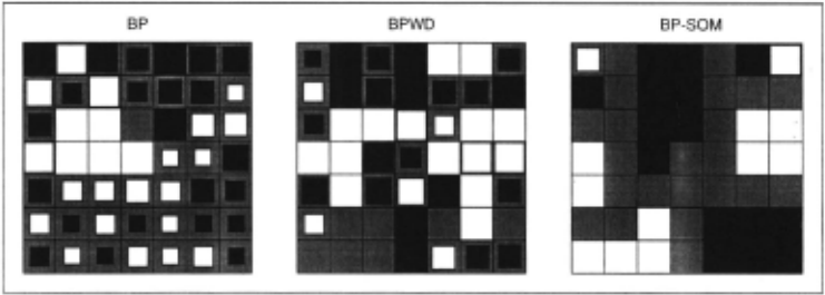
To visualise the differences between the representa tions developed at the hidden layers of the MFNs trained with BP, BPWD, and BP-SOM, we also trained SOMS with the hidden layer activities of the trained BP and BPWD networks. The left part of Figure 3 visualises the class labelling of the SOM attached to the BP-trained MFN af ter training; the middle part visualises the SOM of the BPWD-trained MFN, and the right part displays the SOM of the BP-SOM network after training on the same ma terial. The SOM of the BP-SOM network is much more organised and clustered than that of the SOMs corre sponding with the BP-trained and BPWD-trained MFNs. The reliability values of the elements of all three SOMs are represented by the width of the black and white squares. It can be seen that the overall reliability and the degree of clusteredness of the SOM of the BP-SOM network is con siderably higher than that of the SOM of the BP-trained and BPWD-trained MFNs.
Third experiment: gene-splice detection
A third comparative experiment was performed by us ing the gene-1, gene-2, and gene-3 benchmark data sets extracted from the Proben1 benchmark collection (Prechelt, 1994). The three data sets are different par titionings of a large data set representing the task of detecting splice boundaries between DNA exons and in trons on the basis of a window of 60 DNA sequence ele ments (nucleotides). Each data set features 1,588 train ing instances, 794 validation instances, and 793 test in stances. The MFN used in the BP, BPWD, and BP-SOM experiments contained 120 input units, 2 hidden units, and 3 output units (the optimal numbers of units as reported in Prechelt, 1994). The size of the correspond ing SOM was set to 3 x 3. The three bottom rows of Table 1 display the generalisation performances of BP , BPWD, and BP-SOM on the three gene tasks, again in dicating a clear advantage of BP-S OM over BP. For all three data sets, the generalisation performance of BP-SOM was significantly better than that of BP (gene1: t(19)=5.65, p<0.001; gene-2: t(19)=4.86, p<0.001; gene-3: t(19)=6.05, p<0.001). BP-SOM also performs significantly better than BPWD on test material (gene1: t(19)=3.79, p<0.001; gene-2: t(19)=8.60, p<0.001; gene-3: t(19)=4.09, p<0.001). Nevertheless, the differ ences between classification errors on training and testing material for all three algorithms indicate that neither BP, nor BPWD, nor even BP-SOM succeed in fully avoiding overfitting.
3.2 Pruning of hidden units
By including V.<nn_e··or in the error signal during BP SOM learning, the hidden-unit activation patterns asso ciated with the same class tend to become more similar. When looking at the hidden-unit activations in BP-SOM networks, we observed an additional effect, viz. that hidden-unit activations culminated in switching between two or three values, or resulted in having a stable activ ity with a very low variance. This clearly contrasts with hidden units in MFNs trained with BP , of which all acti vations usually display high variance. To illustrate this phenomenon, Figure 4 shows the standard deviations on training material of the 20 hidden-unit activations of an MFN trained with BP (top row), BPWD (middle row), and BP-SOM (bottom row) , all three algorithms trained on the parity-12 task (1,000 instances). The standard devi ations of ten of the twenty units in the BP-SOM network are equal to 0.01 or lower.
Whenever a unit has a stable activity with a low stan dard deviation for all training instances, it is redundant in the input-output mapping. In that case, the unit can be pruned from the network. Its effect on the following layer (i.e., its mean activation multiplied by its weights to units in the following layer) can be included in the weights from the bias unit . This pruning can be per formed both during and after training.
We trained BP , BPWD, and BP-SOM on the date calculation task and the parity-12 task, attempting to prune hidden units according to a threshold criterion during training. (The gene-splice task was not included because only two hidden units were used in the MFN.) We introduced a stability threshold parameter s, denot ing the standard deviation of the unit's activation below which it is pruned. After a number of pilot experiments with different values for s, we performed experiments with s = 0.01 . All three algorithms were trained on each of the two tasks with ten different random initialisations.
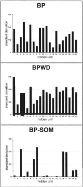
We found that BP-SOM was able to prune 8 out of 25 hidden units for the case of the date-calculation task, and 12 out of 20 hidden units for the case of the parity-12 task (in both tasks, it is an averaged result over 10 ex periments), without loss of generalisation performance. With the same setting of s, trained on the same tasks, no hidden units could be pruned with BP, nor with BPWD. Only with s = 0.1 hidden units could be pruned dur ing BP and BPWD learning; however, this led to seriously worse generalisation performance of these networks.
4 Conclusions
We have shown that BP-SOM has been able to avoid overfitting for the date-calculation task and also for the parity-12 task. Moreover, it outperforms BP and BPWD when dealing with the gene-splice detection task, al though on this task it does not succeed fully to avoid overfitting. Furthermore, BP-SOM is shown to increase the amount of hidden units that can be pruned without loss of generalisation performance. These improvements are due to the cooperation in BP-SOM between supervised and unsupervised learning; i.e., its ability to guide clus ters of hidden-unit representations associated with the same class to be more similar to each other. The highly varying hidden-unit representations of MFNs trained with BP and BPWD are simplified by BP-SOM learning to repre sentations with limited activation values. This reduction of complexity occurs during learning, which enables the pruning of hidden units (the reduction of the size of the network) during learning.
@inproceedings{ijcai1997p165,
  title     = {Avoiding Overfitting with BP-SOM},
  author    = {Weijters, Ton and van den Herik, H. Jaap and van den Bosch, Antal and Postma, Eric O.},
  booktitle = {Proceedings of the Fifteenth International Joint Conference on
               Artificial Intelligence, {IJCAI-97}},
  publisher = {International Joint Conferences on Artificial Intelligence},
  editor    = {Martha E. Pollack},
  pages     = {1140--1144},
  year      = {1997},
  note      = {Neural Networks},
  url       = {https://ijcai.org/proceedings/1997/165},
}
TY - CPAPER TI - Avoiding Overfitting with BP-SOM AU - Weijters, Ton AU - van den Herik, H. Jaap AU - van den Bosch, Antal AU - Postma, Eric O. T2 - Proceedings of the Fifteenth International Joint Conference on Artificial Intelligence, IJCAI-97 PB - International Joint Conferences on Artificial Intelligence PY - 1997 SP - 1140 EP - 1144 UR - https://ijcai.org/proceedings/1997/165 ER -Copied
Machine-readable versions of this paper, for tools and AI agents:





