Unbiased Assesment of Learning Algorithms

1 Introduction

Estimating the accuracy of a classifier is a topic that has experienced much attention in the ML community. One of the main results is that N -fold cross validation pro­ vides a bias-free [Sto74] though not variance-free [Zha92; Koh95], estimate of the true accuracy. n-fold cross validation means that n classifiers are learned from ((n- 1)/n)ths of the available data, and tested on the remaining (1/n)th of the training set. The averaged ac­ curacies are a bias-free est imate of the accuracy of a classifier that is learned by the same algorithm on the complete data set. If the data set is too large, the accu­ racy is usually estimated on a test set that was not used for learning (one-shot training and test), which causes a slight pessimistic bias. For model selection purposes, a .632 bootstrap [Efr79] may be preferable. Bootst rap experiments are conducted by re-sampling a number of training sets of size n from an original data set of size n by randomly drawing samples with replacement. On the average, (1- 1/e)m R:: .632m distinct samples will ap­ pear in the training set, and the averaged accu racies on the remaining test sets provide an opt imisticall y biased estimate. The variance is claimed to be lower in many cases than the variance of cross validation [Efr83], which is important when choosing an optimal model.

Many papers propose new or modified machine learn­ ing algorithms, with claims such as "my new algorithm B is way better than algorithm A", or "extension X im­ proves algorithm A a lot" typically supported by ranking experiments on a well known set of benchmark problems. There is also a book [MST94], resul ting from the Euro­ pean StatLog project, that is dedicated to the compari­ son of learning algorithms for benchmark problems .

Virtually any learning algorithm possesses a number of parameters (e.g., learning rates, number of learning steps , pruning thresholds, etc.). Selecting values for these parameters is the model selection task, which has to be considered a part of the training process. Unfortu­ nately, it has become custom to adjust these parameters such that the error on either the test set, or, in case of n-fold cross validation, the averaged error on the n test sets, is minimized . Since the error on the test set is used as the quali ty criterion for the model selection task, the test set influences the training process. Hence, the as­ sumption that the test sets are not used for learning , which is essential to the result that n-fold cross valida­ tion is bias-free, is violated.

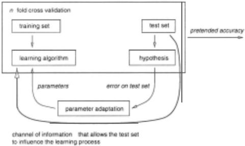
Many authors are aware of that problem and prop­ erly separate model selection from accuracy est imation, e. g. , [KJ97], but a majority of authors seem to consider the resulting distortion of the results negligible. One of many examples is the StatLog proj ect [MST94], where it has not been taken into account by all contributing part­ ners. A slight bias would not be dramatic, if all learning algorithms would be effected equally, such that ranking results would still remain valid . But we argue that the parameters form a communication channel from the test set to the learning algorithm (see Figure 1) , and that the resulting bias depends on the capacity of this channel, i.e., the number of parameters, and the number of different parameter settings which are tested. The main reason why many authors conduct their experiments in the naive way is that unbiased experiments imply a lot of additional computational effort, especially when the parameters are manually adjusted. Our main contribu­ tion is to quantify this parameter-bias, identifying some cases where it actually is negligible and showing others where it makes ranking results invalid.

In the following sections, we consider different experi­ mental settings: Section 2 quantifies the bias of one-shot training and test, Section 3 quantifies the bias of n-fold cross validation when different parameters are used for each of the n trials, and Section 4 is dedicated to cross validation with equal parameter settings for each of the n trials. Section 5 finally recalls the proper way of con­ ducting ranking experiments.

2 One-shot training and test

In this section, we assume the following setting. A learn­ ing algorithm L accepts a set of parameters and there are 2P distinct parameter settings (i.e., the algorithm pos­ sesses logb(2P) parameters with b possible values each). This set of parameters can be viewed as a communica­ tion channel from the parameter optimizer to the learner with a capacity of p bits.

2.1 Communication

As Figure 1 illustrates , when the learner is presented a set of parameters and a training set, it generates a hypothesis h which is used to determine the accuracy of h on the test set of size m . The parameter optimizer is told this accuracy and responds with a new set of parameters, which are again used for training. This cycle is repeated t times, and the best observed accuracy on the test set is then submitted for publication. Based on the accuracy measured on the test set, the parameter optimizer can send p bits of information on the test set to the learning algorithm.

If H is the entropy of the test set then the capacity of the parameter channel allows to transmit information about the class labels of c = y test samples (because H bits are required to encode the class label of one sample), e.g. , if the test set contains 4 uniformly-distributed class labels , the entropy will be 2, allowing a parameter chan­ nel of width 4 (16 distinct settings) to transmit the class labels of 4/2 = 2 test objects. This leaves two questions to be answered: how does the parameter optimizer get to know the class labels of the first c test instances, and how much will this knowledge improve the result?

2.2 Parameter adjustment

The parameter optimizer guesses parameters and obtains the accuracy on the test set in return. We assume that the learning algorithm passes these parameters to the hypothesis, which uses the information to classify the first c test objects that it encounters in some particular way, i.e., the parameters encode class labels for the first c test objects. Then the parameter optimizer can use the following strategy:

1. for all objects i, 1 through c
2. (a) for all labels l, 1 through !classes!
3. tell the learner to classify the ith object as class l and determine the accuracy acc1
4. (b) keep the label of i to the class value l * that resulted in the highest accuracy acc1·

This algorithm tries the assignment of every possible class label to each of c test samples, resulting in a com­ plexity of c · !classes! learning trials, and finds the pa­ rameter setting that encodes correct class labels for c samples. We can view this algorithm as greedy search for optimal learning parameters , but since the correct class label of sample i is independent of the assigned class label of any other sample, the greedy algorithm will find an optimal assignment after c ·!classes! trials 1

2.3 Increase in observed accuracy

Now, after being told the class labels of the first c test objects, how much can we hope to improve the accu­ racy on the test set? Assume that we have an initial classifier h, learned by C4.5 [Qui92] say, which classi­ fies Ph objects of the test set (of size m) correctly. For the first c test instances we repeat the class labels that we were told by the parameter optimizer, rather than using h, we classify the remaining m - c instances us­ ing h. Hence the number of hits is Ph - x + c, where x is the number of hits that h would have obtained on the first c test instances (which are now classified cor­ rectly). We now determine the probability P( c- X 2: z) that this procedure increases the number of hits by z . Drawing c samples from a total of m, we know that Ph of the m are "hits" (classified correctly by h). Hence, the number of hits within the c drawn samples follows a hyper-geometric distribution (note that m is finite). We then replace the c drawn samples with c "hits" (because the parameter optimizer "tells" us their class labels via the parameter channel) .

1 Note that this is not a lower bound for the number of trials, as we have found an algorithm that needs only c( ~ - ~c + n) - n trials in the worst case, but while the algorithm given above essentially performs a gradient search in parameter space, the faster algorithm behaves unlike we would expect a parameter optimizer to behave, so the first result should be somewhat closer to the behavior of a "real" learning algorithm.

This leads us to the bias and computational effort (ex­ plained in Section 2.2), required to achieve this bias for one-shot training and test. t is the expected number of learning experiments that need to be conducted in order to obtain Ph + z hits on the m test samples with prob­ ability P( c- X 2: z), when Ph is the true hit rate of h, provided a parameter channel with p bits of capacity is used.

2.4 Affected benchmark problems

In this section, as well as in Sections 3.1 and 4.1, we will quantify the bias on concrete data sets. We assume that we use a real learning algorithm, C4.5 in most cases, which we "tune" with additional parameters in order to pretend to outperform the learning algorithm one rank higher than the initial learner. We will answer two ques­ tions: How many parameters do we need to succeed with probability > 90% after performing sufficiently many tri­ als (note that this is an exact rather than an empirical result) and how many trials do we need in the average to obtain this result , provided the parameter optimizer performs gradient search in parameter space, which may be an inexact result since it depends on the actual opti­ mizer as well as how strong the parameters influence the result.

Land-sat satellite images: This data set contains 4435 training and 2000 test instances. The default er­ ror rate is .231. Based on [MST94], C4.5 is ranked lOth (error .150, i.e.,l700 hits on the test set) . To be ranked 9th it would have to outperform Bay-tree (error .147) for which C4.5 needs only z = 6 extra hits on the test set . If we get class labels of c = 60 instances , then P(c- X 2: z) > 90%. Hence we need t = 6' 60 = 360 trials with different parameter settings and since H = 2.5 we need a parameter channel of 150 bits. Although an automatic parameter adjustment system may very well run 360 trials, a parameter channel of 150 bits is fairly uncommon (e.g., achieved by 45 parameters with 10 pos­ sible values each). Using c = 16 samples (parameter channel of 40 bits) and 96 experiments, we still have a 2% chance of being over-ranked .

DNA: This data set, also described in [MST94], pos­ sesses 2000 training and 1186 test instances. C4.5 is ranked lOth (1096 hits) . To be ranked 9th it would have to outperform INDCart, requiring z = 4 extra hits. We need to be told c = 85 class labels to achieve this with 90%: P(c- X 2: z) > .9. Since we have 3 classes , we need t = 3 · 85 = 255 trials. Since H = 1.4908, we need 126 bit of parameters, e.g., 37 parameters with 10 possible values each .

For both data sets we conclude that only a very ea­ ger scientist may obtain a modest over-ranking of his algorithm by using an incremental algorithm and an au­ tomatic parameter-adjustment procedure.

3 n-fold cross validation with parameter adjustment

In this section we study the bias caused by parame­ ter adaptation when n-fold cross validation is conducted with parameter values chosen differently for the n runs of the learning algorithm. As an example, the number of learning steps is crucial to the performance of back prop­ agation. Often, the optimal number of learning steps is determined by observing the error on the test set and selecting the point at which the error rate starts increas­ ing again. The minimum errors that occured in the n learning curves are then averaged and published, i. e.,t.he number of learning steps may not be fixed to one value within the n folds. Also, this setting is often used when the splits of the training set are explicitly stated (e.g. , mesh or vehicle silhouettes).

To achieve an average of z extra hits per fold this way, n · z has to equal at least nc - I:; X; , where X; is the number of hits lost by not using h on c samples of fold

Unfortunately, there is no explicit formula for the dis­ tribution of a sum of hyper-geometric random num­ bers. However, we can split the probability of a sum of random numbers considering every possible combina­ tion that yields this sum [Ren70] : P(X + Y = z) = L:j P(X = j)P(Y = z- j) . We can use this equation to split the last summand, resulting in the following recur­ sive equation: P(L:;:1 X; = x) = L:}=o P(L:;:~ 1 X; = x - j)P(Xm = j) . Instantiated to our situation this yields

Straightforward evaluation of this recursive equation for an instantiation is very expensive, since for each evalua­ tion of P(l::7=1 X; = k) we must calculate P(L:7;1 1 X; = k') for every k' < k. By iteratively filling an array that is indexed n and k with P(l::7=1 X; = k) the formula can be evaluated quickly.

3.1 Affected benchmark problems

FEM mesh design: [DM94], a relational problem pop­ ular in inductive logic programming. It is explicitly split into five learning problems. There are 277 samples and 13 classes and he entropy is H = 2.87. FOIL [Qui90] achieves an accuracy of 21% (59 hits). To achieve 26% accuracy with a probability of 99%, FOIL needs c = 5 class labels, while to achieve 31% with a probability of 93% FOIL would need c = 8 class labels. To achieve

26%, we need to conduct 65 trials and a parameter chan­ nel of 14 bits, while to achieve 31% we require 104 trials and a parameter channel of 23 bits.of The parameter adaptation bias is so strong, that accuracy results can easily be pushed from 21% to 31% on this data set.

Diabetes: There are 768 samples with 2 classes, H = .9331. C4.5 achieves 561 hits (rank 13), we need to outperform Quadisc (.5 additional hits per fold). We only need c = 4 class labels to succeed with probability 92%, i.e.,we need a parameter channel of 3.7 bits and have to conduct 8 trials .

In this experimental setting (parameter optimization in each of the n folds) almost arbitrarily good results are easily achievable. Ranking results achieved with this setting are distorted with high probability.

4 n-fold cross validation with fixed parameters

While in the last section the parameter optimizer was able to communicate the class labels of the first c test objects to the learner, the best the parameter optimizer can do here is to communicate the most frequently ob­ served class label of test object i in all folds for the first c objects. If, for example, we have 3 folds and in two of them the first presented test object is of class A, the parameter optimizer may tell the learner that the first presented test object is of class A, which entails 2/3 of an extra hit averaged over the three folds.

Now what is the probability that the number of extra hits Y gained this way takes value y? We study this problem for two class labels. In this case, for each posi­ tion in the test set j, 1 ~ j ~ c, we choose the class that the majority of the n samples (drawn from position j of the n folds) belongs to. There will be max { y , n - y} rep­ resentatives of this class. Assuming that cis significantly less than m and the probability of choosing y samples is binomially distributed B(n,p)(y), where pis the proba­ bility of the default class, i.e., the most frequent class in the data set 2 . Hence:

The total number of nz additional hits on n folds is the difference between the number of extra hits as explained in the last paragraph and the number of lost hits by not using the hypothesis h calculated in the last section:

2 Without this assumption the probability would be hyper­ geometrically distributed, but the number of parameters needed to determine the class labels of a number of samples that gets close to the size of the test set would be outrageous.

We can determine P(I:;j= 1 Yj = l) and P(I:;7=1 X; = l - k) as follows:

Note that in this situation the probability of being ranked too high depends on the hit rate of a default classifier and the hit rate of the initial hypothesis: if the default hit rate is high and the initial classifier performs poorly, the probability of being over-ranked is high.

4.1 Affected benchmark problems

Diabetes: In this setting, we need c = 7 parameters to achieve .5 extra hits per fold with a probability of 2%. Increasing the number of parameters further decreases the probability, since the expected number of samples with equal class labels at some position in n folds, di­ vided by the number of folds, is small compared to the hit rate of the initial hypothesis. In this experimental setting, diabetes is "safe".

Heart disease: In this data set [MST94] there are 270 samples, 2 classes, H = .991. Since C4.5 performs poorly for this problem we only need c = 2 extra hits, a parameter channel of 2 bits and 4 trials are sufficient to succeed with > 90%. If we use k-NN as true learning algorithm (16 hits per fold), we need 6 extra hits to be ranked one rank better. With c = 9 samples, we succeed with probability of 90%. This is due to the fact that the default probability is not much worse than our initial hypothesis. We need a parameter channel of 8 bits and have to conduct 18 trials. We see a strong bias on this data set.

5 Unbiased assessment

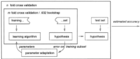
In this section we want to review how unbiased ranking experiments are supposed to be conducted. What has to be kept in mind is that model selection must not be con­ fused with accuracy estimation . The impact of this well known result on accuracy estimation of parameterized learning algorithms has to be realized. As Figure 2 il­ lustrates, parameter adaptation needs to be performed without considering the test set. In order to get a reliable estimate of the optimal parameter settings, m-fold cross validation or .632 bootstrap should be conducted. The best parameter setting is then used to learn a classifier on the whole training set, and the hypothesis is assessed on the test set. In order to get an unbiased estimate, n-fold cross validation has to be conducted making n · m learning trials in total. Averaged over sufficiently many learning problems, this procedure clearly grants an un­ biased estimate of the average performance of a learning algorithm, but it may be painful, since n · m trials need to be conducted for each problem.

6 Discussion

Our calculation clearly shows that adapting the param­ eters such that the accuracy on the test set is optimized causes an optimistic bias that depends on the number of parameters and the number of trials. We quantified the bias that will be observed when sufficiently many trials are conducted and the learner makes optimal use of the available parameters, and we calculated the ex­ pected number of trials needed, assuming the parameter optimizer follows a gradient descent-like search.

It shows that it is hard to be over-ranked in the one­ shot training and test situation if the test set is large. In the n-fold cross validation situation, the probability of being over-ranked is high if the difference between de­ fault hit rate and true accuracy is low. If in the n-fold cross validation setting different parameter values are used (i.e., the parameters are optimized locally) a highly over-ranked result can be achieved, so experiments con­ ducted this way do not yield valid results.

Our considerations do not prove that any learning al­ gorithm actually is much worse than claimed, but they do show that such claims are not validly supported by experiments in the naive setting. Our results are con­ structive in some sense: using the provided equations it can easily be proven that in some situations - depending on the properties of the data set - the naive but inexpen­ sive experimental setting yields perfectly valid results.

Based on our calculations, the validation of perfor­ mance evaluations for new learning algorithms seems to be difficult: many authors do not document their ex­ perimental settings to a sufficient degree, and empirical results that are based on the naive setting are likely to be distorted and cannot be compared to those obtained with unbiased experiments. Heuristic modifications that add new parameters may easily be over-estimated. Even if the modification does not improve the true accuracy of the hypothesis, a new parameter may improve the ranking results.

An important question is which additional assump­ tions were made in our calculation. To summarize them: we assumed that the test sets are in random order (in contrast to ordered by their class labels), but that the order is fixed, as experiments with different parameter settings are conducted. We also assumed that the pa­ rameter optimizer conducts a gradient descent for op­ timal parameters and showed that it will find optimal parameters if the parameters encode class labels for the first c test samples. Hill climbing algorithms for parame­ ter adaptation are fairly common. Also, different param­ eter settings will result in different classification of some of the test samples, although not every distinct parame­ ter setting may yield a different classifier. However, the correlation between parameters and class labels of test set samples is usually less direct than assumed, hence the number of experiments required to gain z extra hits may be higher, and-depending on the learner- the bias may be smaller in real world situations than in our cal­ culation.

Parameters of learning algorithms are undesirable since the more parameters an algorithm has the less ro­ bust the algorithm is, and the harder it is to obtain a satisfactory result for a new problem. Buchanan, para­ phrased by [Cat91], called this the China syndrome:

Some learning algorithms have so many parameters that the only person who can make the program run is with high probability currently in China. Here we have illus­ trated the following extension of this syndrome, which might be considered Murphy's law on machine learning algorithms: the algorithm that is ranked most highly, and is therefore considered most suitable for a given problem, is the one that is least likely to run and grant a satisfactory result because it has so many parameters that the only person who claims to be able to make it run is, with high probability, currently unavailable.

Acknowledgment

This work was supported by a grant of the DFG. We wish to thank Prof. Alberto Segre who did a great job of helping us to edit this paper, and Prof. Wysotzki for the interesting discussion.