Sparse Constraint Graphs and Exceptionally Hard Problems

1 Introduction

It has been observed by several authors in recent years, beginning with Cheeseman, Kanefsky and Taylor [Cheeseman et al., 1991], that for many types of prob­ lem where a large population of problem instances can be examined, there is a phase transition as a problem parameter is varied. The phase transition is from a re­ gion where almost all problems have many solutions, and are relatively easy to solve, to a region where almost all problems have no solution, and are relatively easy to prove insoluble. The intervening region, where the probability that a problem is soluble falls from close to 1 to close to 0, is termed the mushy region [Smith, 1994; Smith and Dyer, 1995]; as the problem size increases, the mushy region becomes increasingly narrow, and in the limit there is an instantaneous phase transition from solubility to insolubility. Within the mushy region, prob­ lems are on average hard to solve, or prove insoluble: it has been observed experimentally that the peak in av­ erage difficulty occurs at the crossover point [Crawford and Auton, 1993], where the probability that a problem is soluble is 0.5.

· Stuart Grant is partly supported by a studentship from British Telecom plc.

It has been observed by [Hogg and Williams, 1994] in graph colouring problems and by [Gent and Walsh, 1994] in satisfiability problems, that although there is a well­ defined peak in the median cost to find a solution in the region of the phase transition, this is often not where the hardest individual instances occur. Given a large sample of problems, individual problems which are very hard to solve may occur in the region where most problems are relatively easy to solve. These problems may be so hard that their cost significantly affects the value of the mean cost; it is for this reason that authors reporting phase transition behaviour have often used the median rather than the mean as a measure of average difficulty.

This paper presents experimental investigations into these exceptionally hard problems occurring in the easy region, in the case of binary constraint satisfaction prob­ lems (CSPs). In this paper, a problem instance is said to be an exceptionally hard problem ( ehp) for a particular search algorithm if:

1. it occurs in the region where almost all problems are soluble, and on average easy to solve (that is, outside the mushy region);
2. it is much more difficult, by at least an order of magnitude, than almost all other problems with the same parameter values;
3. it is more difficult than almost all the problems oc­ curring in the mushy region.

This is intended to be a description of ehps, rather than a precise definition. As will be seen, the individ­ ual ehps that we have found are highly dependent on the algorithm being used: even a minor change in vari­ able instantiation order may convert an ehp into a much easier problem. So although individual ehps, and what makes them so difficult for a particular algorithm, should be investigated, we can also ask about ehps in relation to populations of problems and in relation to search al­ gorithms: for instance, do ehps occur in all populations of problems, and are some search algorithms more sus­ ceptible to ehps than others?

2 The random generation model

The experiments reported here were done using randomly-generated binary CSPs. Each set of problems is characterized by four parameters: n, the number of variables; m, the number of values in each variable's do­ main; Pt, the proportion of pairs of variables which have a constraint between them (i .e. the constraint density); and P2, the proportion of pairs of values which are in­ consistent for a pair of variables if there is a constraint between them (i .e. the constraint tightness).

When constructing the constraint graph, we choose Ptn(n- 1)/2 of the possible variable pairs at random; for each selected pair there will be a constraint between the corresponding variables. For each constrained pair of variables, we choose m 2 p2 of the possible pairs of val­ ues, at random, to be the pairs forbidden by this con­ straint. The phase transition from under-constrained to over-constrained problems is observed as p2 varies, while n, m and Pt are kept fixed; below, sets of randomly­ generated problems with fixed n, m and p1 and varying P2 will be referred to by the tuple ( n, m, p1).

Many of the experiments described later involve sparse constraint graphs (i .e. with small p1). The problem gen­ erator described above will then produce a proportion of disconnected graphs. Since a problem with a discon­ nected graph would in practice be dealt with by solving the subproblems separately, we did not include discon­ nected graphs in our samples. If the problem generator produced such a graph, it was rejected and a new graph generated, until a connected graph was found.

For most of these experiments, the problems were solved using the forward checking algorithm with a vari­ able ordering heuristic using the fail-first principle: the first variable to be instantiated is the one which is most constrained, and thereafter, the next variable to be in­ stantiated is one with fewest remaining values in its do­ mam.

3 Where do ehps occur?

Figure 1 shows the results of a set of experiments with n = 20 and m = 10 and the constraint density, p1 , equal to 1.0, 0.7, 0.5, 0.3 or 0.2. 1 For each value of p1 , a range of values of P2 was chosen , so as to cover the crossover point and the region of increasing average difficulty leading up to it. In order to have a reasonable chance of seeing the extremes of behaviour, 1000 problems were generated at each set of values of the four parameters. The cost of solving each problem was measured by the number of consistency checks required to either find one solution or prove the problem insoluble.

'We did not c.onsider Pt = 0.1, as we did in later ex­ periments with n = 50, because, as already described, the constraint graph had to be connected, and connected graphs

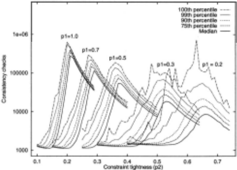
Following the graphs shown by [Hogg and Williams, 1994) and [Gent and Walsh, 1994), Figure 1 shows anum­ ber of higher percentiles as well as the median for each set of 1000 problems. The behaviour of the median as Pt decreases is as shown in Prosser's extensive series of experiments [Prosser, 1994): the peak median cost coin­ cides with the crossover point, in each case, but as the constraint graph becomes less dense, the phase transition becomes less sharp. When p1 = 1.0, all the percentile curves are close together; as p1 decreases, they become more widely separated, and the maximum cost begins to behave erratically. To the left of the peak, when p1 = 0.2, the maximum cost is sometimes two orders of mag­ nitude higher than the median.

It is noteworthy that although, in general, as p1 de­ creases, each succeeding phase transition gives rise to easier problems, the single most difficult problem in the whole set of experiments occurs when p1 = 0.2, shown by the 'spike' in the maximum when p2 = 0.63. This problem is insoluble. It is not an ehp by the criteria given earlier, since it is not in the region where most problems are easy: there are, however, ehps when p2 = 0.54 and 0.56, which are both soluble problems. The most difficult problem occurring when p1 = 0.3, at p2 = 0.48, might also be classed as an ehp, although it is on the edge of the mushy region.

These experiments suggest that ehps are not a univer­ sal phenomenon of randomly-generated CSPs, but occur only in sparse problems. Since it is conceivable that ehps would be found in denser problems if the sample sizes were sufficiently large, we have carried out further ex­ periments with (20, 10, 1.0) problems, generating up to 50,000 problems for each value of p2 ; no ehps were found (the results are shown in [Smith and Grant, 1994]). We have also examined larger dense problems ( (20, 20, 1.0) and (30, 10, 1.0)) and found no ehps. If these are typi­ cal, then at the least, ehps in dense problems must be extremely rare compared with those in sparse problems.

with 20 nodes and 19 edges are not very interesting for our purposes.

4 Larger Sparse Problems

As noted in the last section, the phase transition is less sharp in sparse problems than in dense problems, given the same values of n and m. It might be suspected therefore that the ehps seen in the (20, 10, 0.2) prob­ lems were a side-effect of this, and that in larger prob­ lems, as the phase transition becomes more abrupt, ehps would tend to disappear. Figure 2 shows the results of experiments with larger sparse problems: again, 1000 problems were generated for each data point. 2 As ex-

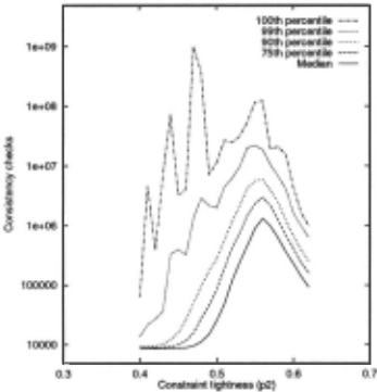
pected, the (50, 10, 0.1) problems show a much sharper peak in the median than the (20, 10, 0.2) problems. The increase in n from 20 to 50 has caused the phase transi­ tion to become more abrupt, even though the density is lower. However, far from disappearing, ehps are if any­ thing more common, and are more extreme, than in the smaller problems.

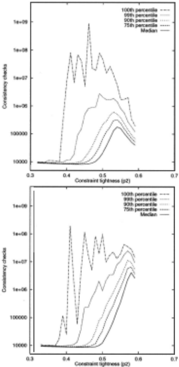
One difference between the set of problems shown in Figure 2 and, say, the (20, 10, 1.0) problems of Figure 1 is that the former includes many different constraint graphs, whereas all the (20, 10, 1.0) problems have the same constraint graph. We considered whether the oc­ currence of ehps depends on the topology of the con­ straint graph. This seemed possible, because it has been shown in [Smith and Dyer, 1995] that the location of the phase transition in randomly-generated sparse CSPs de­ pends on the constraint graph: the more irregular the constraint graph, the lower the value of p2 at which the phase transition occurs. For example, it might be that some constraint graphs give rise to problems which are very susceptible to ehps, whereas others produce more homogeneous behaviour, similar to the denser constraint graphs of Figure 1. The same set of 1000 constraint graphs was used at each value of p2 in Figure 2. We selected the most regular (graph 739) and the most ir­ regular (graph 904), and used each graph as the basis of two new sets of problems, again with 1000 instances generated at each value of p2 : all the problems in one set had constraint graph 739 and all the other set had graph 904.

2 Figure 2 is therefore based on solving 23,000 individual CSPs; it takes hours to solve some of the worst individual problems (on a SPARCstation IPX, using C) and altogether Figure 2 represents well over 100 hours of cpu time.

The results for the two problem sets are shown in Fig­ ure 3. As expected on the basis of previous experience, the peak in the median cost occurs at a higher value of p2 for the more regular graph than for the more irreg­ ular graph. From the higher percentiles, it can be seen that the irregular constraint graph gives more variable behaviour over the phase transition than does the reg­ ular graph. However, it is hard to see any significant difference in the behaviour of the maximum before the phase transition in the two graphs: both graphs seem more or less equally susceptible to ehps.

We also took one of the ehps from Figure 2 (that oc­ curring at p2 = 0.48, with graph 358) and generated a set of problems with this constraint graph. If any randomly­ generated constraint graph is likely to produce more ehps than others, a graph which has already produced an ehp should be a good choice. Graph 358 does not appear to be exceptional in any way, and solving the problems pro- . duced similar results to Figure 2 (shown in [Smith and Grant, 1994]), so that once again, it does not appear to be especially susceptible to ehps.

We have not, therefore, found any randomly-generated sparse constraint graphs which do not produce ehps, nor any which appear to be more likely than others to give rise to them. A more thorough investigation, consider­ ing a wide range of constraint graphs and much larger sample sizes, might show that the incidence of ehps is higher for some constraint graphs than for others, but since ehps are by definition rare and difficult to solve, this would be a daunting task.

5 Anatomy of an ehp

To understand better the causes of ehps, we examined carefully the three ehps shown in Figure 2, i.e. the most difficult problems at p2 = 0.44, 0.47 and 0.48. For these values, the median cost is about 10,000 consistency checks; the easiest of the three ehps takes more than 72

million consistency checks. These values of p2 are well outside the mushy region, and all three problems have solutions. Why, then, are they so difficult to solve?

One of these problems is problem 358 at p2 = 0.48. The first four instantiations made by the forward check­ ing algorithm are v5 = 1, 3 v16 = 4, v22 = 9, v37 = 4. It (eventually) becomes clear that this set of as­ signments leads to an insoluble subproblem. However, proving insolubility takes more than 376 million con­ sistency checks; the algorithm frequently finds partial solutions with 38 or more variables instantiated before detecting an infeasibility and backtracking. Once it has been proved that there is no solution to the subproblem, the alternative assignment of v37 = 10 is tried and leads almost immediately to a solution. Since only one possi­ ble instantiation of the first variable, v5, has been tried, it is very likely that this problem has many solutions.

In the other two ehps, similarly, the first few assign­ ments lead to a subproblem which has no solutions, and almost all the search effort is expended in proving this. Partial solutions involving most of the variables are found in the course of searching the subproblem re­ sulting in a great deal of backtracking. As with problem 358, the solutions eventually found for these two prob­ lems have the first variable assigned its first value, so that there are very probably many solutions in other ar­ eas of the search space. We have seen the same kind of behaviour in other ehps which we have found.

3 i.e. variable 5 is assigned the value 1.

These results are very similar to the experience re­ ported by [Gent and Walsh, 1994]; they found a sat­ isfiability problem which required more than 350 mil­ lion branches to solve, using a simplified version of the Davis-Putnam algorithm. The first choice made by the algorithm led to a very difficult unsatisfiable problem, which required almost all the search effort; the alterna­ tive choice led immediately to a solution. They conclude that: "These difficult problems are either hard unsatis­ fiable problems or are satisfiable problems which give a hard unsatisfiable subproblem following a wrong split."

It appears that, in CSPs also, ehps are problems in which the search algorithm gets into a hard insoluble subproblem early in the search. All the ehps that we have seen in these experiments are themselves soluble; if an insoluble problem were to occur at these values of P2 it would be extremely hard to prove insoluble, since a complete exploration of the search space is required. However, it seems that ehps of this type are exceptional even amongst ehps.

6 Can ehps be avoided?

There are, in theory, two potential ways of avoiding ehps which arise through encountering insoluble subproblems early in the search: one is to avoid getting into such sub­ problems in the first place, and the other is to find some search algorithm which can detect that the subproblem is insoluble more quickly.

In the problems we have considered, clearly the in­ soluble subproblem would have been avoided if a differ­ ent instantiation order had been chosen, or if a different value had been chosen for one of the variables. How­ ever, it seems unlikely that different ordering heuristics could eliminate ehps altogether: they might avoid par­ ticular instances that the fail-first heuristic encounters, and so find those problems easy to solve, but might then meet insoluble subproblems in other problems that the fail-first heuristic would avoid.

The alternative is to search the insoluble subprob­ lem more quickly. An obvious candidate for considera­ tion is some kind of informed backtracking, rather than chronological backtracking as in the basic forward check­ ing algorithm. [Prosser, 1993] describes an informed backtracking algorithm, conflict-directed backjumping (CBJ), and shows that it can be combined with for­ ward checking (FC) to produce a new search algorithm, FC-CBJ. In his experiments with the zebra problem, he showed that FC-CBJ was the best of the algorithms that he considered, including plain FC: on individual in­ stances, FC-CBJ almost always did better than FC and was never worse.

We have used both algorithms in combination with fail-first, as described earlier: these will be termed FC­ ~F and FC-CBJ-FF. Figure 4 shows the results of apply­ mg FC-CBJ-FF to the problems which were previously solved using FC-FF to produce Figure 2. It is evident

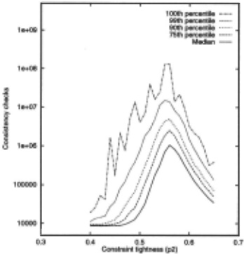
that CBJ does significantly reduce the difficulty of ehps for this population of problems: the most difficult prob­ lem in the easy region, at P2 = 0.52, takes 39 million consistency checks, which is much less than the three ehps from Figure 2 considered earlier.

Problem 358 at P2 = 0.48 and problem 898 at p2 = 0.47 were ehps for FC-FF because the first four variable instantiations led to an insoluble subproblem: since we are using the same variable and value ordering heuris­ tics with FC-CBJ-FF, the same subproblems are en­ countered. These problems are not ehps for FC-CBJ­ FF precisely because the algorithm can detect that the subproblem has no solutions much more quickly than chronological backtracking can. There is a vestige of the earlier difficulty with problem 358: FC-CBJ-FF takes more than 3 million consistency checks to prove insolubil­ ity and this is one of the most difficult problems at that value of P2· Problem 898, on the other hand, which was the most difficult of all the problems plotted in Figure 2, taking more than 10 9 consistency checks, succumbs to CBJ quite quickly: the subproblem is proved insoluble in only 150,000 consistency checks.

Hence, using an informed backtracker such as CBJ instead of chronological backtracking moderates the dif­ ficulty of ehps, but does not eliminate them altogether. It remains an open question whether any algorithm will be able to eliminate ehps entirely from the populations of sparse CSPs that we have considered.

7 The benefits of CBJ

If Figures 2 and 4 are compared, it can be seen that they are very similar, apart from the 99th and 100th percentiles. This suggests that CBJ's biggest effect is on the most difficult problems, and that its performance is otherwise similar to chronological backtracking, when combined with FC and FF.

Figure 5 shows the cost of solving a problem using FC­ FF compared with the cost using FC-CBJ-FF when p2 = 0.48, where FC-FF encounters one of the ehps considered earlier (problem 358). The 1000 problems which were

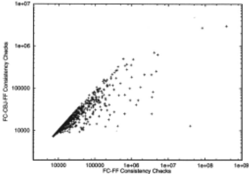
generated with these parameter values for Figures 2 and 4 are plotted as individual points in Figure 5, although most of them cannot be distinguished. The median cost is 10786 consistency checks for FC-CBJ-FF, 11235 for FC-FF, and for well over half the problems, the perfor­ mance of FC-CBJ-FF is not very different from that of FC-FF. It is only for the 100 or so most difficult problems that there is a dramatic difference in cost between the two algorithms. Similar plots for other values of p2 con­ firm that FC-CBJ-FF does not offer great savings over FC-FF except for the most difficult problems occurring before the phase transition.

These findings to some extent contradict Prosser's· he found that on average FC required about 3.5 time~ as many consistency checks as FC-CBJ. However, Prosser used a fixed instantiation order, rather than the dynamic order given by FF. It appears that most of the benefit of using CBJ in conjunction with FC can be obtained more simply by using the fail-first heuristic, perhaps because, for most problems, the ordering given by fail-first en­ sures that chronological backtracking usually results in backtracking to the real culprit for a failure, so that in­ formed backtracking does not add very much. Since CBJ carries an additional overhead, which is not reflected in the count of consistency checks, 4 it may be that for some regions of the parameter space FC-FF would be a bet­ ter choice. For instance, we have compared the two al­ gorithms on the problems shown in Figure 1, and for p1 ~ 0.5, the number of consistency checks is identical in almost every instance. However, for sparse problems, FC-CBJ-FF does offer a great benefit in overcoming the most difficult problems in the region where most prob­ lems are easy and soluble.

4 We have found that FC-FF can do about 8% more con-

8 Discussion

We have shown that when the constraint density is high, there is much less variation in problem difficulty at a given value of the constraint tightness than when the constraints are sparser. As a corollary of this, we have found no instances of ehps except at low constraint den­ sities, from samples of up to 50,000 problems with each set of parameter values. Whether ehps might arise even when the constraints are dense, given sufficiently large sample sizes, remains an open question. In sparse prob­ lems , the incidence of ehps does not seem to depend greatly on the constraint graph, although it is difficult to be sure from the small numbers of ehps that we have found .

It should be noted that our graphs exhibiting ehps show no sign of the double peak in the higher percentiles found by [Hogg and Williams, 1994]. However, their ex­ periments, on 3-colouring problems, used far larger sam­ ples than ours; they had between 10,000 and 1 million samples for each data point, and were thus able to see smooth behaviour in the 99.95 percentile. We have in­ creased our sample size to 10,000, at considerable cost in cpu time, without seeing any sign of a double peak, but if it were feasible to solve 1 million samples in cases such as the (50, 10, 0.1) problems considered earlier, the double peak might then appear.

We have shown that ".dding an informed backtracker (CBJ) to forward checking and the fail-first heuristic can make a huge difference to the difficulty of ehps; CBJ al­ lows the algorithm to search insoluble subproblems much more quickly than a chronological backtracker can do. Ehps thereby become much less significant, but do still occur.

However, except for the hard problems in the easy re­ gion, and in particular the ehps, CBJ does not give great savings over chronological backtracking, when applied to sparse problems. With dense problems, our experiments suggest that it is not worthwhile to use CBJ at all, in conjunction with FC-FF.

It should be remembered, however, that all our exper­ iments are based on random problems generated by the model described earlier. Problems with more structured constraint graphs, varying domain sizes and/or varying constraint tightness might well behave differently. How each of these factors might affect the incidence of ehps, or the performance of the algorithms we have considered, has yet to be explored.

sistency checks per second than FC-CBJ-FF.

This paper illustrates that the full story of the relative performance of two algorithms needs to be based on a wide range of problems, including the extremes of prob­ lem difficulty. Judging by the median cost alone, FC-FF is at most 60% more expensive than FC-CBJ-FF, on the (50, 10, 0.1) problems. However, on some of the hard problems, the performance of FC-CBJ-FF is orders of magnitude better than FC-FF; this would be sufficient to give a considerable difference in the mean cost of the two algorithms at these points. In order to be able to design a comprehensive set of experiments comparing different CSP algorithms, it is therefore essential to con­ sider phase transition behaviour, and, in particular, the existence of occasional exceptionally hard problems.