
Experiments with Associative-Commutative Discrimination Nets
Proceedings of the Fourteenth International Joint Conference on Artificial Intelligence. Automated Reasoning. Pages 348-354.
© 1995 International Joint Conferences on Artificial Intelligence
Abstract
We recently proposed a data structure, called associative-commutative discrimination nets, that supports efficient algorithms for (manyto-one) term matching in the presence of associative-commutative functions. In this paper we discuss the integration of such discrimination nets into an actual equational theorem prover and report on corresponding experiments. The general associativecommutative matching problem is known to be N P-complete, but can be solved in polynomial time if the given terms are linear, i.e., do not contain multiple occurrences of the same variable. We therefore have implemented a two-stage matching procedure. First we check whether a match exists for the linearized versions of the given terms (where different occurrences of the same variable are replaced by different new variables). If a match for the linearized terms does exist, we then determine whether there is also a match for the original, non-linear terms (i.e., whether the proposed substitutions for different occurrences of the same variable are consistent). Our experimental results indicate that this approach works very well in theorem proving, where most matching attempts actually fail and are filtered out during the first stage, so that the second, more expensive stage of the algorithm is only needed in comparatively few cases.
- [Bachmair et al., 1993] L. Bachmair, T. Chen, and lv Ra- makrishnan. Associative-commutative discrimination nets. In Proceeding8 of the 4th International Joint Confer• ence on Theory and Practice of Software Development, CAPP/FASE, pages 61-74, Orsay, France, April 1993. Springer-Verlag LNCS 668.
- [Benanav et al., 1987] D. Benanav, D. Kapur, and P. Naren- dran. Complexity of matching problems. Journal of Sym- bolic Computation, 3:203-216, 1987.
- [Christian, 1989] J. Christian. High-Performance Permuta- tive Completion. PhD thesis, The University of Texas at Austin, August 1989.
- [Forgy, 1982] C. Forgy. Rete, a fast algorithm for the many patterns many objects Match problem. Artificial Intelli• gence, 19:17-37, 1982.
- [Graf, 1994] P. Graf. Extended path-indexing. In 1!Uh Con- ferenec on Automated Deduction, pages 514-528. Springer- Verlag LNCS 814, 1994.
- [McCune, 1992] W. McCune. Experiments with discrimination-tree indexing and path indexing for term retrieval. Journal of Automated Rea8on- ing, 9:147-167, 1992.
- [Ohlbach, 1990] H.J. Ohlbach. Abstraction tree indexing for terms. In Proceeding8 of the 9th European Conference on Artificial Intelligence, pages 479-484, London, August 1990. Pitman Publishing.
- [Papadimitriou and Steiglitz, 1982] C. H. Papadimitriou and K. Steiglitz. Combinatorial Optimization: Algorithm8 and Complexity. Prentice Hall, 1982.
- [Ramesh et al., 1990] R. Ramesh, I.V. Ramakrishnan, and D.S. Warren. Automata-driven indexing of prolog clauses. In Seventh Annual ACM Sympo8ium on Principle8 of Pro- gramming Language8, pages 281-290, San Francisco, 1990.
References were extracted automatically from the PDF and may contain errors.
Full text extracted automatically from the PDF; figures, tables and equations may differ. The PDF is the version of record.
1 Introduction
Matching and unification are two fundamental opera tions in theorem proving. Unification is part of deduc tive inference rules such as resolution, whereas matching is needed for subsumption, normalization by rewriting, and other mechanisms for simplifying formulas and elim inating redundancies. Experimental evidence indicates that the efficiency of resolution-type provers mainly de pends on these simplification mechanisms. For instance, in rewrite-based equational theorem provers, most of the time {about 80 to 90%) is spent on term rewriting and normalization-operations that both require matching- Siva Anantharaman Jacques Chabin Departement d'Informatique LIFO, Universite d'Orleans 45067-0rleans Cedex 02 (France)
and relatively little on deducing new formulas via unifi cation. In resolution-type theorem provers the deletion of subsumed clauses is critical for performance. In short, efficient implementations of matchin~ are indispensable for such provers, cf. [McCune, 1992j. We should also point out that pattern matching algorithms are a key component in many other applications, including func tional and logic programming [Ramesh et al., 1990) and rule-based expert systems [Forgy, 1982).
It is becoming increasingly clear that many applica tions of theorem proving. require efficient methods for reasoning about associative-commutative functions. In this paper we discuss our work on extending the equa tional theorem prover REVEAL by efficient algorithms for matching in the presence of associative-commutative function symbols.
2 Preliminaries
We consider terms built from function symbols and vari ables. The letters 8 and t are used to denote terms, f and g to denote function symbols, and z, y, and z to denote variables. The expression tjp denotes the subterm oft at position p. Positions may, for instance, be represented in Dewey decimal notation. The top-most position is de noted by A, and hence tJA = t. The sequences 2 and 2.2 denote positions in t = f(a, g(a, b)), with tJ2 = g(a, b) and tJ2.2 = b.
Let AC be a set of associativity and commutativity 8.XlOmS
for some function symbols f. We also write f E AC if f is such an associative-commutative symbol and write 8 = AC t to indicate that 8 and t are equivalent under associativity and commutativity. A term t is said to AC match another term 8 (and 8 is called an AC -instance of t) if there exists a substitution u, such that tu =Ac s.
It is convenient to represent terms equivalent under AC by flattened terms. Let L be the set of all rewrite rules {called flattening rules)
where f E AC, and X, Y, and Z are sequences of terms with JXJ+JZJ :2: 1,JYJ :2: 2. {By JXJ we denote the length of a sequence X.) Terms that can not be rewritten by L are said to be flattened. The flattened version of a term t is denoted by t. By ...., we denote the smallest symmetric rewrite relation (also called the permutation congruence) for which
iff E AC. It is readily seen that a is an AC-instance oft if and only if tu ...., s, for some substitution u. (In the case of flattened terms, we have to allow zu to be a sequence of terms if z occurs as an argument of an AC-symbol in t.)
3 Discrimination Nets
Various data structures have been proposed for the el ementary operations needed in theorem proving, e.g., [Ohlbach, 1990; Graf, 1994]. We illustrate the basic ideas by way of an example for one such data structure discrimination nets-and its use for matching, or more specifically many-to-one matching, where one wishes to identify, given terms t 1, ... , tn (called the patterns) and 8 (called the subject), which of the terms ti match a. In rewrite-based theorem proving, the terms ti represent the left-hand sides of the current rewrite rules, whereas the subject term a is the term to be rewritten. This matching problem needs to be solved for several differ ent subject terms, but with a fixed set of patterns. For instance, many terms may need to be rewritten using the same set of rewrite rules. Therefore, the pattern terms are represented by a special data structure similar to a trie and called a discrimination net, that allows one to quickly identify matching patterns for any given subject term. A key idea is that common parts of terms ti be shared in the representation of the full pattern set.
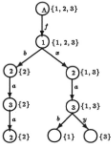
For example, suppose we have three pattern terms, f(z, a, b), f(b, a, a), and f(z, a, y). A discrimination net T for the set M of these three patterns is shown in Fig ure 1. The discrimination net is a tree, with edges la belled by function symbols and variables (occurring in terms in M) and nodes labelled by positions (of sub terms of terms in M) and subsets of M. The labelling needs to satisfy the condition that for each node u, the associated set M.,. consists of exactly those terms in M
with occurrences of function symbols as prescribed by the path from the root of the net to u. (The sets M.,. are called match sets for obvious reasons.) Interior nodes indicate partial matches, and leaves, complete matches.
For example, the left-most leaf in the net in Figure 1 has match set {2}, as t 2 = f(b, a, a) is the only term in M which has an f at the root (position A), a b at position 1, and an a at positions 2 and 3.
To determine which patterns match a given terms a one simply traverses the discrimination net with the in put term a as a guide. More specifically, an edge is tra versed if its label is either identical to the corresponding symbol in 8 or else is a variable. For example, the term a = f(a, a, a) causes traversal of the rightmost path in T, which yields match set {3} and indicates that a is an instance ofts, but not oft1 or t 2 · The traversal induced by the term f(b, b, b) gets stuck at the second level, in dicating that there is no match.
3.1 Associative-Commutative Discrimination Nets
Let us next consider how discrimination nets may be applied to terms with associative-commutative function symbols. By the AC -nesting depth of a position in a term we mean the number of AC-symbols that occur on the path from the position to the root. More formally, the AC-nesting depth at A is 0; and if n is the AC nesting depth at position p in t, then the AC-nesting depth at a position p.i in t is n + 1, if t contains an AC symbol at position p, and n, otherwise. The AC-nesting depth of a term is the maximum AC-nesting depth of any of its positions. The top-layer i of a term t is the expression obtained from t by removing all subterms at positions with non-zero AC-nesting depth. For example, iff E AC and g ~ AC, then the top-layer of g(z, f(b, c)) is g(z, f). Obviously, if a is an AC-instance oft, then its top-layer must be an (ordinary) instance of the top layer oft. For example, the term g(a, g(a, a)) cannot be an AC-instance of g(z, f(b, c) as the respective top layers do not match. If the top-layers of the given terms match, we need to consider the stripped-off subterms and recursively check for the existence of suitable AC matches.
Thus, if a and t are flattened terms with tu ...., a, then (i) i matches 8 and (ii) if p is a position of an AC-symbol in the top-layer oft, then (tip)u...., sip· Con versely, if (i) and (ii) are satisfied for some substitution u, then tu...., a. In other words, AC-matching is completely characterized by conditions (i) and (ii). Condition (i) represents a standard matching problem, while condi tion (ii) leads to a bipartite graph matching problem. Suppose tip= f(t 1 , ··· ,tm) and sip= f(sl, ... ,sn), where f E AC. We may also assume, without loss of generality, that the terms t1, ... , t1c are non-variables, while all terms tlc+l· ... , tm are variables, for some k with 0 ~ k ~ m. Define a bipartite graph G = (V1 u V2 , E), with V1 = {s1, ... ,sn}, V2 = {t11 ··· ,t~c}, and E con sisting of all pairs (ai, t;), such that t;u...., si, for some substitution u. It can easily be seen that if (a) either n = m or n > m > k, and (b) there is a maximum bipartite matching of size k in the bipartite graph G, then /{t1, ... , tm)u"' f(8t, ... , 8n), for some substitu tion u and hence condition (ii) is satisfied. In part (a), if m > k, then some of the terms ti contain variables and, since we consider linear pattern terms only, a suitable matching substitution can be found, whenever all non variable terms t1, ... , t1c are matched (and n 2: m, of course). For example, iff E AC, then 8 = f(h(a), a, b) is an AC-instance oft = f(h(z), y): substitute a for z and the sequence a, b (or f(a, b)) for y.
These observations lead to the definition of an AC di8crimination net for a set of terms M as a hierar chically structured collection of standard discrimination nets: the top of the hierarchy is a standard discrimina tion net for the set of top-layers of terms in M; to each node with an incoming edge labelled by an AC-symbol (a so-called AC -nodes) another AC-discrimination net is attached that represents the sub terms of terms in L,., where Lu is the set of terms corresponding to the AC node.
For example, an AC-discrimination net for the two terms k(f(a,b),c,J(y,c)) and k(f(a,z),c,J(a,b)) where f is the only AC-symbol, is shown in Figure 2. Both
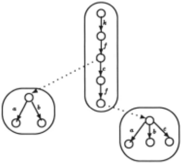
terms have the same top-layer, k(f, c, !). The set of terms {f(a, b), f(a, z)} is associated with the first AC node; the set {f(y, c), f(a, b)} with the second AC-node. The corresponding subnets represent {a, b} and {a, b, c }, respectively.
To determine which terms AC-match a given term 8 1 we traverse the individual standard nets in the hierarchy as usual, and use a bipartite graph matching algorithm to combine the results from different levels of the hier archy. For example, suppose k(f(b, a), c, f(a, b)) is an input term for the above AC-net. The top-level net is successfully traversed to the first AC-node, call it v, at which point the two subterms band a are provided as in puts to the first subnet (which represents the terms a and b). Traversal of the subnet yields two bipartite graphs, one for each element of the set L.., = {! (a, b), f (a, z)}. The size of each respective maximum matching indicates that the input term f(b, a) is an AC-instance of both f(a, b) and f(a, z). Traversal of the top-level net resumes at node 11 and continues on to the second AC-node, call it v', with £..,, = {f(y, c), f(a, b)}. The input terms for the second subnet are a and b. The subterm f(a, b) of the input is found to be an AC-instance of f(a, b), but not f(y,c). Thus, only the pattern k(f(a,z),c,f(a,b) is identified as an AC-match. A full description of the algorithm can be found in [Bachmair et al., 1993].
3.2 Secondary Automata
The AC-matching algorithm has to construct bipartite graphs of the form G = (V1 u V2 , E), where V1 = { 8t, ... , 8n} is a set of input sub terms, V2 = { t1, ... , t11} is a set of (non-variable) pattern subterms, and E con tains an edge (8i, tj) if and only if tj AC-matches 8i, so as to extract subsequently a maximum matching of size k. The set V2 depends only on the patterns; it re mains fixed for a given AC-net and node therein and, at least for applications in theorem proving, is usually small with at most five elements. The set of vertices V1 and the set of edges E depend on the input. The graph G is computed stepwise, via a sequence of bipartite graphs Gt, ... , Gn. Traversal of the subnet for input 81 deter mines the edges incident on that node, thereby defining G1. Traversal of the subnet for 82 determines the edges incident on 82 , which are added to G1 to yield G2 ; and so on.
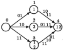
For example, consider V2 = {tt, t 2}. Each traversal of the subnet for a term 8i yields a bitstring bi of length two: the bitstring 10 is obtained if 8i is an AC-instance oft1 but not oft2 ; and the strings 00, 01 and 11 are inter preted correspondingly. The size of a maximum match ing on the bipartite graph Gi can be readily determined from bi and the size (and kind) of a maximum matching on Gi-l· The computation can be conveniently repre sented in a finite automaton, which we call a secondary automaton. More specifically, we speak of a secondary automaton of rank k (denoted by S~c) if V2 contains k elements.
The secondary automaton S2 is shown in Figure 3.2. The initial state of the automaton represents graphs with a maximum matching of size 0; its three successor states represent three different types of graphs with maximum matchings of size 1; 1 and the final state represents graphs with a maximum matching of size 2. In our algorithm we use secondary automata up to rank 5, which is sufficient for theorem proving applications.
1 The three cases are: (i) h can be matched, but not t 2 ; (ii) t2 can be matched, but not t1; (iii) both t1 and t2 can be matched, but not at the same time.
4 Implementation of AC-Matching
The AC-matching problem is an N P-complete problem, but can be solved in polynomial time if pattern terms are linear [Benanav et al., 1987]. We have therefore designed AC-matching as a two-phase process. In the first phase, an AC-discrimination net for the linearized versions of patterns is used as a filter: if no AC-match exists for the linearized patterns, then there certainly exists none for the original patterns. If in the first phase some terms are identified as AC-matches, we need to check in a second phase whether any of these matching terms can be ex tended to AC-matches in the presence of non-linearity. A straightforward AC-matching algorithm is used in this second phase. Our experimental results provide strong evidence that in typical theorem proving problems most of the patterns can be eliminated during the first phase, so that the expensive second phase is invoked only spar ingly and the two-phase approach results in substantial performance gains.
4.1 Term representation
We adopt a variant of the data structure for flat terms used in HIPER, see [Christian, 1989] for details. Flat tened versions of terms equivalent under AC are unique only up to permutation congruence. For instance, the two terms f(a, b, c) and f(c, a, b) are AC-equivalent if f E AC. We define a unique representative for each AC equivalence class by using a total ordering on function symbols and variables and lexicographically extending it to a total ordering on terms. The minimal term in an equivalence class serves as the unique representative. For example, if a< b < c, then f(a, b, c) < f(c, a, b).
4.2 Standard Discrimination Nets
Let us next discuss the design and implementation of dis crimination nets. We first consider standard discrimina tion nets, which provide the basis for AC-discrimination nets. In theorem proving, the set of (pattern) terms that need to be represented in a discrimination net change dy namically. We have chosen a non-deterministic variant of such nets in which insertion and deletion of patterns can be performed easily. (The main difference between deterministic and non-deterministic nets is that the lat ter require backtracking in order to identify all matches. Deterministic nets require no backtracking, but may use more space.)
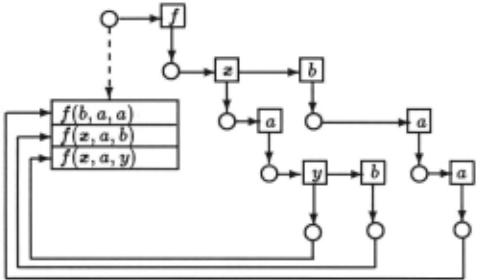
Pattern terms are stored at the root of the net. Each leaf maintains a list of pointers to the patterns in the matchset associated with the leaf node. With each node we maintain a linked-list representing the (labelled) edges from that node. This list is kept sorted (according to the edge labels), so that the traversal of the net can be implemented by a linear search through this list.
Example 1 Figure 4 6how6 the di6crimination net for the 6et {f(z, a, b), f(b, a, a), f(z, a, y)}, where the under lying ordering on 6ymbol6 i6 z < y < a < b < f.
This variant of discrimination nets essentially corre sponds to the third variant described in [McCune, 1992]. In contrast to HIPER and also our earlier description of discrimination nets in [Bachmair et al., 1993], we distin guish between different (non-AC) variables. Although such a distinction may potentially result in more back tracking and consume more memory, it has the advan tage that checking for the consistency of substitutions for (non-AC) variables can be done during traversal of the net, so that failures caused by inconsistencies can be discovered earlier. To allow for consistency checking we maintain a global substitution table and, whenever descending to a branch corresponding to a (non-AC) variable z, compare the entry for z (if present) in the substitution table with the current sub term of the input term.
4.3 AC-Discrimination Nets
Recall that AC-nets require additional operations such as bipartite matching using secondary automata, inter section of matchsets produced by AC-subnets and re porting the result from one level of the net to the next higher level. We first describe data structures that are needed for these operations. With each AC-node v we associate a set L .. of AC-subterms. These subterms are stored in a linked list; each element in the list is called a control block and corresponds to one AC-subterm. In the control block for a term t E L .. we maintain information relevant to bipartite matching and secondary automata transitions. When a pattern term is deleted, all control blocks corresponding to its AC-subterms must also be deleted. To facilitate deletion, each pattern is assigned an unique ID number and all control blocks derived from the pattern inherit this ID, which is then used as a search key during deletion. The search is implemented as a sim ple linear search in the linked list associated with L .. .
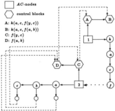
For each pattern, there is a pointer from the control block of each AC-subterm tat AC-nesting depth l to the control block of an AC-superterm 2 oft at AC-nesting depth l- 1. Similarly, if a term tis-in the matchset of a leaf, there is a pointer from the leaf to the control block of the closest AC-subterm enclosing this t.
Example 2 Suppo6e k(a, c, f(y, c)) and k(a, c, f(a, b)), f E AC, are two pattern6. We have L2 {f(y, c), f(a, b)} repre6ented by the li6t of control block6 C and D. The enclo6ing AC-6ubterm of f(y, c) and I( a, b) are the patterns themselves. So there is a pointer from control block C to A and D to B.
2 An AC-superterm of t is a superterm of t with AC function symbol at its root.
L---------------------.J
Figure 5: AC-discrimination net
4.4 Secondary Automata
A secondary automaton is constructed for each desired rank and stored during initialization of the system. Each state of a secondary automaton is implemented as an ar ray of pointers. Recall that transition symbols are bit strings. We use the integers representing the bitstrings as indices with the arrays. For example, Figure 6 is the secondary automaton of rank 2 (also see Figure 3 for its abstract representation) where each state is represented as a four-element array. On bitstring 01, whose integer value is 1, the automaton changes from state 0 to state 1.
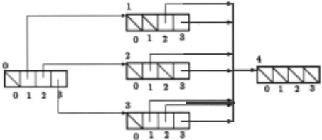
Bitstrings are obtained as follows. Note that for a pattern l(tl, ... , t~c, Zlc+b ··· , zm), I E AC, and a sub ject l(s1 , .·· ,s,.), each Si, 1 ::=; i ::=; n, can AC-match more than one t;, 1 ::=; j ::=; k. Since nondeterministic nets are used, t; may appear in the matchsets of dif ferent leaf nodes, all of which will be visited when Si is being matched. We assign each t; a bitstring of length k such that the bits for the bitstring for t; are all ze ros except the lh bit. The input bitstring to the sec ondary automaton for Si is then obtained by performing an inclusive-OR operation between the bitstrings oft;, where t; is in the matchset of a leaf node visited. For instance, for the pattern l(h(a,z),h(a,c),e), IE AC, the arguments h(a, z), h(a, c) and e are in matchsets of different leaf nodes, say node 1, 2 and 3, and the bit strings associated with them are 100, 010 and 001, re spectively. On the subject l(h(a,c),e,e), since h(a,c) AC-matches with both h(a, z) and h(a, c), leaf nodes 1 and 2 will be visited and so the bitstring obtained will be 100 V 010 = 110, indicating that h(a, c) matches the first and second arguments of the pattern.
Opthnization to reduce rank: The number of non variable arguments of an AC-subterm in a pattern deter mines the rank of the associated secondary automaton. The size IS~c I of a secondary automaton grows rapidly with increasing k. For instance, IS1I = 2, IS2I = 5, !Sal = 16, IS41 = 68 and ISsl = 406. We only con struct secondary automata up to rank 5, but this has not been a limitation in practice. In particular, we use optimization techniques that have enabled us to run all the benchmarks using automata of rank ::=; 5. First ob serve that multiple occurrences of the same term can be merged for the purpose of constructing secondary au tomata. We only need to keep track of the multiplicity of each distinct argument. For instance, to deal with the sub terms in I( a, a, b, c, c, c) we only need an automaton of rank 3, not rank 6. Also, we may partition terms according to their top function symbol. For example, suppose t1 = k(tD, t2 = k(t~), ta = k(t~), t4 = h(t~), t 5 = h(t~), and t6 = h(t~). Evidently, an instance of one of the first three terms can not be an instance of one of the last three terms, and vice versa. Consequently, in stead of using an automaton of rank 6 for all six terms, we may use two automata of rank 3 for each of the two subgroups. If necessary, we can partition further by look ing at more function symbols other than the top symbol.
4.5 Putting it all together
We are now ready to explain the operation of an AC discrimination net based upon the above representation. At each AC-node, we do the following steps. We check whether (i) the number of arguments in the pattern ex ceeds those in the subject; or (ii) if the pattern has no variable arguments and has fewer non-variable argument than the subject. In such cases, the pattern is marked unmatchable and no further action is done on behalf of it. For patterns which pass the above test, secondary automata are used to determine the existence of a maxi mum bipartite matching for the corresponding bipartite graph. Secondary automata are used for small bipar tite graphs (deriving from pattern terms with few non variable AC-arguments). If the number of non-variable arguments is large, we use a general bipartite matching algorithm [Papadimitriou and Steiglitz, 1982]. In the ex periments reported below, we never had to resort to a general bipartite matching algorithm.
On successful completion of the above steps, we in clude the AC-subterm in the matchset for the AC-node. This matchset is intersected with those computed at other AC-nodes at the same level of the net. We use Stickel's algorithm [McCune, 1992] to do list intersec tion. Specifically, suppose L1 , L2 and La are three lists.
We first mark the elements of L1 with 1. Then those elements of L2 that are marked with 1 are marked with 2. Finally, elements of La that are marked with 2 are the results of L1 n L 2 n La. Since an intersection has to be done at each AG-node, we can use the number of AC-nodes visited for each level as the current value of the mark. Finally, when a leaf node r is reached, the matchset M,. associated with r is also intersected with the outcome of earlier intersections at this level.
Example 3 With the AC-discrimination net in Fig ure 5, suppose the subject is k(f(a, c), c, f(a, b)) and we have just entered node 2. Upon processing f(a, c) through the subnet at node 2, only B is marked with 1, since f( a, z) of the second pattern is matched, but not f( a, b) of the first pattern. Then, although both terms f(a, b) and f(a, b) in La are in the matchset computed at node 3, only B gets marked with 2 because it is marked cur rently with 1. Therefore, the second pattern is selected by the net.
5 Experimental Results
We next present experiment~ results we obtained with our implementation on a Spare 10 with 32 MB of mem ory. We first compare AC-discrimination nets with straightforward AG-matching, and then show the ef fect of the resulting savings in the context of a the orem prover. Finally, we show that the use of AC discrimination nets does no compromise on the perfor mance of a theorem prover on problems without associa tivity and commutativity.
5.1 AC-Matching
The first data set provides an indication of the effec tiveness of AG-discrimination nets. We took a set of 1 000 terms from a typical theorem proving application ~ OTTER [McCune, 1992), and built an AG-net for it. Then each one of these terms is used as a subject (resulting in a successful AG-match, of course). The re sulting times are compared with a straightforward AG matching algorithm that uses no discrimination net. We ran the algorithms in two different modes: (i) to identify the first matching term (and then stop), or (ii) to find all matching terms. We also repeated these tests for a smaller subset of 100 terms.a The results are summa rized in Table 1. It can be seen that AG-discrimination nets result in a three- to four-fold speedup for finding the first matching term (which is the variant needed for rewriting). All times are in seconds.
5.2 AC-Completion
We then ran a number of experiments with our equa tional theorem prover REVEAL. All problems contain.ed associative-commutative function symbols. They m clude the following:
- grobner: The Grobner base of a certain ideal in a poly nomial ring in two variables over integers is computed via completion;
3 We should note that the terms in the original OTTER examples do not contain AC-symbols; but we declared one of the (binary) symbols to be AC.
| Problems | Net | No Net | With Net | Speedup |
|---|---|---|---|---|
| CLpos_100 First | 0.02 | 8.38 | 1.05 | 7.98 |
| All | 8.83 | 1.08 | 8.18 | |
| CL_pos_1000 First | 0.15 | 43.74 | 11.48 | 3.81 |
| All | 87.62 | 11.44 | 7.65 | |
| CL..neg_100 First | 0.03 | 0.48 | 0.15 | 3.20 |
| All | 0.93 | 0.12 | 7.75 | |
| CL..neg_1000 First | 0.47 | 45.45 | 12.74 | 3.57 |
| All | 89.63 | 12.20 | 7.35 |
- grpfini30: A canonical rewrite system is computed for an abelian group of order 30, specified with three gen erators;
- jacobson: Commutativity is proved for rings satisfying X 3 =X;
- moufang: The sesquilinearity of the associator is proved for (non-associative) alternative rings;
- robbinh : It is proved that any Robbins algebra is a Huntington algebra (and hence a Boolean algebra) if there exists an element c, such that c + c = c ;
- robbinh2: Similar to robbinh, but under the assumption that there exist elements c, d such that c + d = c ;
- uqsl2 : Certain properties of some 'unitary quantum groups' are proved
Table 2 summarizes timings for these and several other AG-problems. We compare the performance of the prover with AG-discrimination nets (under columns 'ACN' in the table) with a more naive strategy 'Nai' without AG-nets. One of the key components of our prover is the normalization of terms by rewriting, which requires (AC- )matching. Given a set T of rewrite rules and a term 8 to be normalized, the prover takes one rule from T and tries to match it at the root of 8. In case of failure, the next rule in T is tried, and so on, until either a match is found or else all rules in T are exhausted. In the latter case, the process is restarted at the next position of 8. We measured (a) the time to normalize terms with respect to the current rewrite system and (b) the total time leading to proofs. The speedups are given for both the normalization and for total comput ing times. The speedups for normalization, naturally, are significantly greater than those for total times.
Since the prover needs to find only one matching pat tern, from Table 1 we may expect -an average speedup of about 4 for finding the first matching pattern. Since in normalization about half the time is spent in find ing a match, we can expect to improve normalization by a factor of 2 on the average. This is consistent with the speedup figures for normalization in Table 2. Fi nally, about 70% of the total computing time is spent in normalization and the rest on other operations, such as unification (for deduction of so-called critical pairs), etc. So we can expect a speedup of about 35% on the average for completion. This is again consistent with the speedups in Table 2 we obtained for our examples.
| Time | Speedup | |||||
|---|---|---|---|---|---|---|
| Normalization | Total | |||||
| Pro b. | N81 | ACN | Nai | ACN | ||
| balukas | 1.82 | 1.40 | 3.15 | 2.75 | 1.30 | 1.15 |
| boolston | 1.35 | 0.79 | 2.89 | 2.36 | 1.71 | 1.22 |
| grobner | 18.18 | 6.66 | 30.05 | 18.95 | 2.73 | 1.59 |
| grpfini30 | 2.69 | 1.88 | 7.77 | 7.10 | 1.43 | 1.09 |
| hunt2acm | 91.63 | 95.72 | 118.01 | 121.58 | 0.96 | 0.97 |
| jacobson | 137.34 | 61.06 | 169.94 | 89.75 | 2.25 | 1.89 |
| midlaw | 0.29 | 0.20 | 0.99 | 0.90 | 1.45 | 1.10 |
| moufang | 45.74 | 12.76 | 58.97 | 26.12 | 3.58 | 2.26 |
| newpb | 5.26 | 4.00 | 8.19 | 7.16 | 1.32 | 1.14 |
| newpb2 | 7.07 | 5.67 | 10.99 | 9.63 | 1.25 | 1.14 |
| robbinh | 3.11 | 1.18 | 6.47 | 4.50 | 2.64 | 1.44 |
| uqs12 | 10.15 | 1.38 | 15.35 | 6.74 | 7.36 | 2.27 |
Finally, we like to mention that memory consumption of the AC-discrimination nets for the problems in Ta ble 2 never exceeded the memory required for storing the patterns, i.e., the extra memory needed at most doubled.
5.3 Non-AC Problems
As mentioned earlier, standard discrimination nets have been used quite successfully to solve many-to-one non AC-matching problems. It is critical that the perfor mance of our AC-matching algorithm do not degrade when used for non-AC problems. Table 3 shows that this has been accomplished in our implementation. All the problems in there are non-AC. The second col umn are the timings obtained by standard discrimi nation net while the third column pertains to AC discrimination nets. Observe that the overhead of using AC-discrimination net for non-AC problems is negligi ble.
| Problems | SN | ACN | Ratio |
|---|---|---|---|
| as soc | 0.54 | 0.55 | 0.98 |
| groupl | 0.74 | 0.76 | 0.97 |
| groupr | 0.59 | 0.60 | 0.98 |
| fur tin | 0.83 | 0.85 | 0.98 |
| hunting2c | 14.84 | 15.05 | 0.99 |
| ternary | 4.09 | 4.36 | 0.94 |
6 Summary
In this paper, we have presented the design, implemen tation and experimental results of an AC-discrimination net based AC-matching algorithm. This algorithm has been integrated into the equational theorem prover RE VEAL, which we used for our experiments. Our imple mentation exploits the fact that although AC-matching is N P-complete, it can be solved in polynomial time if patterns are restricted to linear terms. It solves the many-to-one AC-matching in two phases. In the first phase only those patterns are selected that AC-match under the assumption that all (AC) variables are differ ent (i.e., linear). The consistency of the substitutions computed for (AC) variables are checked in the second phase. The experimental results show that a high per centage of patterns are filtered out in the first phase, leaving very few patterns for the more complex consis tency checking in the second phase. For instance, for our benchmark problem uqs12, no more than one pat tern was selected by the AC-discrimination in 98% of the cases (no pattern was selected in 88% and one pat tern in 10% of the cases). We also ran experiments with different search strategies and obtained similar results. In particular, we want to mention that on robbhin2 we were able bring down the total time from 213.5 minutes to 175.5 minutes using AC-discrimination nets. All these results and the speedups we obtained provide strong ev idence that AC-discrimination nets and secondary au tomata are indeed useful tools for significantly improving the performance of theorem provers for AC problems.
Achnowledgements. We would like to thank the anonymous reviewers for their helpful comments. This research was supported in part by the NSF under grants CDA-9303181, INT-9314412 and CCR-9404921.
@inproceedings{ijcai1995p46,
  title     = {Experiments with Associative-Commutative Discrimination Nets},
  author    = {Bachmair, Leo and Chen, Ta and Ramakrishnan, I. V. and Anantharaman, Siva and Chabin, Jacques},
  booktitle = {Proceedings of the Fourteenth International Joint Conference on
               Artificial Intelligence, {IJCAI-95}},
  publisher = {International Joint Conferences on Artificial Intelligence},
  editor    = {Chris S. Mellish},
  pages     = {348--354},
  year      = {1995},
  note      = {Automated Reasoning},
  url       = {https://ijcai.org/proceedings/1995/46},
}
TY - CPAPER TI - Experiments with Associative-Commutative Discrimination Nets AU - Bachmair, Leo AU - Chen, Ta AU - Ramakrishnan, I. V. AU - Anantharaman, Siva AU - Chabin, Jacques T2 - Proceedings of the Fourteenth International Joint Conference on Artificial Intelligence, IJCAI-95 PB - International Joint Conferences on Artificial Intelligence PY - 1995 SP - 348 EP - 354 UR - https://ijcai.org/proceedings/1995/46 ER -Copied
Machine-readable versions of this paper, for tools and AI agents:





