On Bootstrapping Local Search with Trail-Markers

1 Introduction

We study a simple, general framework for search called bootstrap search, which is defined as global search using only local search along with some memory for learning intermediate states as subgoals. Although it has not pre­ viously been studied in detail , this simple search frame­ work with subgoal caching is fundamental to a variety of learning processes at an abstract level. For example, in terms of robot path planning [Latombe, 1991], it is a two-level planning scheme with subgoals being land­ marks of either the workspace or configuration space. In terms of concept learning [Thornton, 1992], it cor­ responds to global concept approximation using only a locally-good extrapolator with subgoals as positive ex­ amples. In terms of case-based planning [Kolodner, 1993], it is having memory for cases and a local search for plan modifications and reuse. In terms of problem solv­ ing, the framework is simply to reduce new problems to previously solved ones using an existing resource-limited problem solver.

*This work has been performed at Sandia National Lab­ oratories and supported by the U.S. Department of Energy under Contract DE-AC04-94AL85000.

In this paper, we present a bootstrap search algorithm, and develop some theory on its performance. Our pre­ sentation is in the context of problem solving. More con­ cretely, we use the widely-studied 15-puzzle [Barr and Feigenbaum, 1981], the tile-sliding puzzle with 15 tiles on a 4 by 4 tray, as a motivating example. Thus, given the availability of a local search procedure (e.g., a search algorithm with some maximum time cutoff), we aim to study some ways of bootst-rapping it into a global search using the memory of previously solved problems. Specif­ ically, we characterize the effectiveness of the resulting global search and compare the relative capabilities. Fur­ ther, if the local search is parameterized by some re­ source bound, we also provide a way of approximating the optimum resource bound so that an optimal local search may be used to yield the best global search.

Our work is similar to adaptive path planning [Chen, 1995; 1992], which studies the framework of improving an existing global path planner using a local path plan­ ner augmented with experience. The difference is that bootstrap search does not assume the availability of a pre-existing global searcher, which may be difficult to code or impractical to run. Hence, bootstrap search can be more widely applicable, although it will require more training in general to compensate for the lack of a teacher to provide solutions when local search fails .

Our work is superfacially related to hierarchical Q­ learning [Kaelbling, 1993] in that we both use a land­ mark network; however, our emphasis is on deciding what goals to remember as subgoals rather than which local actions to take. Our work is also related to the use of abstraction and macro-operators [Korf, 1985b], which can be thought of as local methods. However, our emphasis is not on learning new macro-operators, but on improving the use of existing ones through new sub­ goals. In this respect, our work is similar to Stepping­ Stone [Ruby and Kibler, 1989], which improves problem solving by learning new subgoal sequences. However, as in adaptive path planning, SteppingStone also relies on the availability of a global planner (brute-force search) to derive new subgoal sequences for a local planner (means­ ends analysis) to follow. Moreover, SteppingStone uses general subgoals that represent subspaces of states. In contrast, we restrict our subgoals to specific states to gain simplicity. This simplicity allows us to develop a more rigorous understanding of the learning processes within the framework, and hopefully will provide further insight into others. Nevertheless, using specified states does have a more acute scalability problem because of the potentially large number of subgoals required.

2 Algorithm

The basic assumption in bootstrap search is that there is an efficient, though only locally effective search pro­ cedure, local, available that can transform (reduce) any state (problem) u to another v if the pair is 'near' by some metric. A greedy method is often sufficient to im­ plement local. A problem v is directly solvable by local if v can be reduced to a goal state. To 'bootstrap' its global effectiveness, local is allowed to remember in memory U past problems that it had solved. These memory entries can be thought of as trail-markers in that each marker can be traced back to a goal state through calls of local. Of course, the more effective local is, the less boot.strap­ ping it needs . The main issue of bootstrap search IS how to selectively remember past solved problems so that fu­ ture problems can still be efficiently solved.

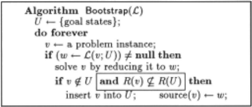
To illustrate, consider the two simple but infeasible algorithms in Figure 1: the first one excludes the boxed fragment, and the second one includes it. We c~ll the first A(O), and the second A(-1). In the algonthms, C is a procedure based on local augmented with mem­ ory U. Upon input problem v, .C goes through U in some order, and returns the first solved problem w to which v can be reduced via local, if w exists; otherwise null is returned. To keep track of the solution paths, a back pointer source( v) for each trail-marker v is maintained.

In A(O), the strategy is to store every solved problem in the past, excluding repetition. Obviously, this strat­ egy will lead to memory explosion, let alone the utility problem [Minton, 1988] of eventual slowdown. Thus, one must stop the training of A{O) eventually and hope that it has received sufficient training. To curb the memory growth, A(-1) requires that the newly solved problem v contribute to the problem solving capability of cur­ rent .C. Given a problem x, let R(x) denote the set of problems reducible to x via local; for a set of problems X, let R( X) denote the union of R( x) over all x in X. Then A( -1) requires that R( v) contain problems not in R(U). Although this requirement will decrease the redundancy within U, it nevertheless cannot be imple­ mented in practice. Hence, we can only use A( -1) for theoretical comparisons.

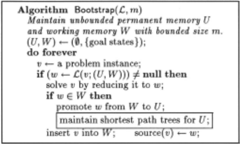
We can be more sophisticated in our learning by aug­ menting U with a working set of trail-markers W. We can selectively remember useful markers by storing tem­ porary markers in W and promoting them into perma­ nent storage U only when they become useful. In Fig­ ure 2, we present A{m), the algorithm parameterized by m, the size of W, using this scheme. The boxed state­ ment does not affect the problem solving capability of .C but should be included when solution quality is an issue.

In A(m), .C checks first through U and then through W for the first solved problem w to which the new prob­ lem v can be reduced via local. If w exists, it is returned; otherwise, null is returned. Thus, if w exists, v is solv­ able by .C and is inserted into W . Learning occurs when wE W, i.e., when v E R(W) \ R(U). In this case, w is 'proven' useful and promoted into U. There is a forget­ ting process dictated by the finiteness of m, which de­ termines the amount of reservoir for storing potentially useful entries. Because v has to be reducible to some current subgoal before it can be stored, the network of trail-markers is always connected. However, the training time required may be more than that of the alternative: Store new problems as potential subgoals even though they may not be currently solvable. This alternative, though, does have its problem of maintaining potentially disconnected network of subgoals.

In C's search through U and W, there may well be additional heuristics available for ordering the trail­ markers for a potential match. Also, search time may be reduced by calling local only when the problem states are deemed sufficiently close by some heuristic measure. Further, portions of U may be skipped to foster more promotions from Wand hence faster learning. However, to keep the algorithm simple and unbiased so that we may understand it more thoroughly, we employ no addi­ tional heuristics. We implement U with an unbounded first-in-first-access list and W with a rotating last-in­ first-access list of size m. The stipulation on U allows us to derive the theoretical predictions later.

3 A Path Planning Example

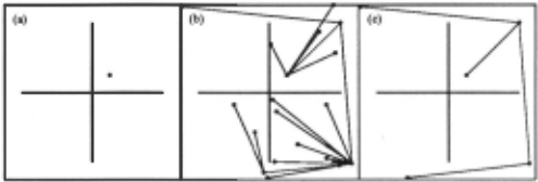
Before applying our algorithm to the 15-puzzle, we first illustrate our algorithm with a simple robot path planning example. Consider a point robot operating in a 4-room workcell as shown in Figure 3a. The workcell is discretized at a resolution of 100 x 100; the center of the dividers is at (0, 0); the lengths of both dividers are 80; and the initial robot 'home' position is at (10, 10) . Suppose that the only path planner available is local, which implements the simple 'go-straight' procedure so that it will succeed if and only if its two given points (starting and ending robot positions) are visible from each other. Using local, which is obviously not complete in this workcell, the robot is to go through a sequence of goal positions drawn uniformly at random. Thus, we need to increase the effectiveness of local.

Note that in adaptive path planning [Chen, 1995; 1992], we have the luxury of having a global searcher to provide a solution whenever the current network of subgoals is inadequate to produce one. In contrast, we do not have such a teacher in bootstrap search. Thus, we need to bootstrap ourselves by learning to achieve easy goals first and use these easy goals to achieve harder goals. Again, the main issue is which goals achieved should be remembered. We should also note that find­ ing a path from the current robot position s to the goal position t is equivalent to finding a path from 'home' to the goal, because s is known to be connectable to 'home' through the current network of sub goals. Hence, we can view the path finding problem in the problem­ reduction framework by identifying the 'home' position as the goal state, and the goal position as the problem state. Further, we may use whatever network learned to accomplish the task of connecting two arbitrary points by connecting them both to 'home' first. Thus, different goal states may be included in the problem-reduction framework by reducing the existing subgoals to the new goal state.

Using our algorithm, it is clearly possible to bootstrap local to total completeness because the workcell is con­ nected under local. The deeper questions are how much training time and memory will be required. Shown in Figure 3b is the graph of the trail-markers learned by a random run of A(O) until it becomes complete. Al­ though in general we cannot know when completeness is reached, we can in this case by testing whether each of the four corners: {(1, 1), ( -1, 1), ( -1, -1), (1, -1)}, are visible from a trail-marker. The figure shows that A(O) required 21 markers, even at the benefit of knowing the optimal stopping time. In contrast, Figure 3c shows the sparsity of the graph learned by a random run of A(1). The number of markers is only one more than the theo­ retical minimum of 4. This 4-fold reduction in memory requirement is obtained at a price, though, of a 5-fold increase in training time: from 29 goals for A(O) to 156 goals for A(1) .

To study the algorithm more, we run A(m) 100 times each, for m = 0,1,2,4,8,16. We also consider different environment complexities by varying the lengths of the workcell dividers d: From d = 80 both, we decrease them both to d = 50, and increase them both to d = 90. The resulting average training time to completeness T and average size of memory at that time S are plotted in Figure 4. Clearly, for m > 0, the fast drop ofT as m increases indicates that having sufficiently large reser­ voir of working memory (e.g., m ~ 8) is important in reducing the training time, but having more than the threshold will not yield much further reduction. More­ over, the lack of variation of S as m increases indicates that the size of working memory has little effect on the size of the final memory learned.

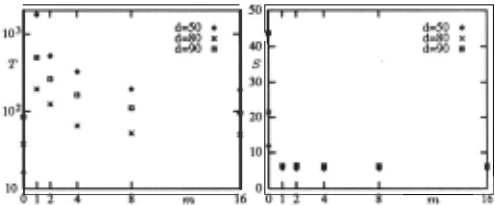
So far there are no surprises. However, as we com­ pare the performance curves of A for different environ­ ments, we see an interesting phenomenon: A can ac­ tually require more training time in a seemingly eas­ ier environment. From the plot of T(m, d), we see that T(O, 50) < T(O , 80) < T(O, 90), confirming the intuition that the shorter the dividers, the easier the environment is to learn. However, form> 0, the plot actually shows on the contrary that T(m, 80) < T(m, 90) < T(m, 50), suggesting that having local more powerful (wider doors implying more local successes) do not necessarily accel­ erate learning, but in fact can hamper learning. The reason for this behavior is due to the greedy nature of A in minimizing S. The algorithm will promote a working marker to permanent storage only when it demonstrates usefulness. Therefore, when operating in an easy envi­ ronment with d = 50, the algorithm can initially learn very quickly markers that will cover most of the workcell, leaving only a small region that is now unfortunately dif­ ficult to learn because goals in that small region will be needed to promote any working marker that is visible from it. For d = 80, the chance of such initial 'over­ learning' is smaller because the doors are narrower . For d = 90, the chance of over-learning is even smaller; but because the doors are now much narrower, learning is significantly slowed. Therefore, as we increase the power of local (doorways widen), we will see the increase of both the chance of learning and the interplaying chance of over-learning.

4 Theory

In this section, we make some precise and strong state­ ments about the performance of our algorithm through mathematical analysis; details of the proofs are provided in the appendix. We first give a sharp bound on the performance of A(O) in Theorem 1 by showing that the 'average' failure probability of .C using its first k trail­ markers decreases exponentially in k. Next, using A(O) as a reference, we show that the performance of A(1) is better than that of A( -1), which is better than that of A(O). The comparison is based on the 'average' fail­ ure probability (or 'average utility' in reverse order) of .C using the first k markers of each algorithm for each k. Finally, we present an upper bound on the 'average' search cost of A(m) for all m in Theorem 3. From this theorem, a technique for finding the best resource bound con local( c) is developed in Section 5.

As in the framework of PAC-learning [Natarajan, 1991], we assume that the problems are randomly drawn from a fixed distribution - in fact , we shall assume a uniform distribution for simplicity. To facilitate our dis­ cussion, we use subscript n on a program variable to denote its value at the nth loop, and parameter m to indicate its correspondence to A(m). Additionally, for k > 0, let Uk be the kth entry to be inserted into mem­ ory U. Thus, R(Un(m)) denotes the set of problems re­ ducible to any of the previously solved and stored prob­ lems in U after A( m) is trained with n problems. The following random variables (with parameter m omitted for notational simplicity) are important in characterizing the learning process.

• An The failure probability of A using Un alone, i.e., the probability that a random problem x does not belong to R(Un), or equivalently, one minus the probability mass on R(Un) ·
• In The 0-1 variable indicating the promotion of Wn+l from W to U on the chance that Vn+l E R(wn+l)\ R(Un), i.e., rwn+l E WnJ, where r·J is the indicator function .
• Ln The amount of additional learning achieved by remembering Wn+l conditional on In = 1, i.e., the probability of a random problem x belonging to R(Un+d but not R(Un), or equivalently, the probability mass on R(Un+d \ R(Un)·

Notice the fundamental equation of An+l = An - Ln In, regardless of m. To study the utility of U, we use index (k) with (0) = 0 to denote the kth n > 0 such that In ~ 1, if it exists; otherwise infinity. Thus, A(o) = 1, A(k+l) = A(k)+l· and A(k) is the failure prob­ ability right before the insertion of Uk+l· Moreover, we have A(k+l) = A(k)- L(k) with L00 ~r 0. Now we in­ troduce a randomized problem model motivated by the 15-puzzle, and study the consequences of this equation under the model.

Definition 1 Let local(c) be a local search procedure with maximum search cost c. A random uniform digraph of problems with edge probability function F( c) is a set of uniformly distributed problems in which every problem using local(c) is independently solvable and reducible to every other problem with probability F(c) .

Thus, the probability that local( oo) will yield a solu­ tion with search cost no greater than cis F(c).

Theorem 1 The average failure probabilities of A(O) when applied on a random uniform digraph of problems of size N decreases almost geometrically in that for all k,

With the performance of A(O) as a reference, the fol­ lowing theorem shows that the utility of memory U(1) is higher than that of U( -1) , which is in turn higher than that of U(O) . In other words, A(1) is better than A( -1) which is better than A(O) in that A(1) will tend tore­ member a more 'compact' set of intermediate solutions than A( -1), similarly for A(O).

Theorem 2 The average failure probabilities of A(1), A(O) and A( -1) when applied on a random uniform di­ graph of problems satisfy

for all k. Consequently, the average failure probabilities of the first k memory entries of the algorithms satisfy

Although the preceding theorem is a strong state­ ment about the relative performance of A(1), A(O), and A( -1), nothing similar is known about A( m) for m ~ 2. We conjecture that A(m) for m ~ 2 is also better than A(O) in that EA(k)(m) ~ EA(k)(O). The following theo­ rem, however, does address the search cost of A(m) for general m.

Theorem 3 For arbitrary m, suppose that we apply A(m) with local( c) on a random uniform digraph of prob­ lems, and that local( c) has conditional expected search cost -y0(c) upon success. Then the expected search cost of A(m) per problem is

Further, suppose that A(m) has failure probability a af­ ter certain amount of training, and that local( oo) has F-tc ) weighted cost 'Yl(a) = fo a zdF(z) for the lower aquantile. Then for the next problem, the expected search cost of A( m) backed up by local( oo) is

5 Application to the 15-Puzzle

To demonstrate, we apply our algorithm and theory to the 15-puzzle. Here, the object is to be able to solve all 16!/2 solvable configurations, though not necessarily in the shortest number of moves. There are of course many different ways of solving the puzzle [Korf, 1985b; Politowski, 1986; Ratner and Pohl , 1986; Ruby and Ki­ bler, 1989]. Since bootstrap search is a weak method, we do not expect it to perform better than other methods that take advantage of additional knowledge. Rather, we use the puzzle to demonstrate the generic applicability of bootstrap search when nothing else is available.

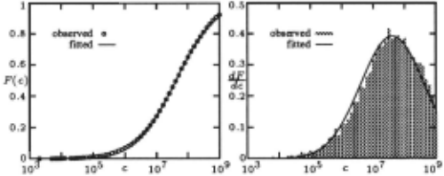
Thus, suppose that we have available only a subrou­ tine local( c), which implements iterative-deepening with Manhatten distance heuristic [Korf, 1985a] and maxi­ mum search cost c, measuring the number of nodes gen­ erated. We ask the question, "Is it possible to bootstrap local( c) (with unlimited amount of training) so that the average search cost is less than that of simply applying local( oo )?" We also ask, "Is it possible to only bootstrap local( c) to a certain degree of capability and back it up with local( oo), so that the average total search cost is less than that of simply applying local( oo )?" As we shall see, the answer to both questions is yes with roughly two orders of magnitude improvement . However, c must be sufficiently large for both cases, and cannot be too large (depending on the desired capability) for the second case. To reach this conclusion, we first need to justify the ran­ dom digraph model and study F(c).

Obviously, the digraph of the solvable states of the 15puzzle induced by local(c) is not random. However, the number of states N = 16!/2 is extremely large and the digraph is almost regular. Hence, it is plausible to model the digraph of the 15-puzzle by the random digraph with F(c) being the fraction of states solvable by local( c). To study this fraction, we apply local(10 9 ) to 10000 ran­ domly generated solvable states, and record the fraction of successes with search cost less than or equal to c, against c as c increases to 10 9 . Since brute-force search costs tend to be exponential, we use log scale on c. We plot loge against the fraction of success under local(c) to obtain the cumulative distribution function and the density histogram in Figure 5. The figure shows that the distribution is in fact approximately lognormal. Us­ ing the quantile estimators [Aitchison and Brown, 1957] (27- 73% for JJ.; 8-92% for u), we estimate that F(c) = A(c I JJ., u), with J-l = 17.536 and u = 2.3436, where A de­ notes the two-parameter lognormal distribution. Thus, let x =loge and x = (lnc-JJ.)/u = (xlnlO-JJ.)/u. Then

is the Normal probability function.

Having approximated F(c), we next describe our boot­ strap search experiment and verify our theoretical pre­ dictions before answering the questions posed in the be­ ginning of this section. For each x = 5, 6, 7, 8, we com­ pare A(1) and A(20) by running them on 10000 random problems. For reference, we also run A(O), but with a pre-chosen bound b on the memory storage: b = 20 for both x = 7, 8; b = 50 for x = 6; b = 200 for x = 5. These bounds are chosen so that storage requirements are comparable to that of A(l) and A(20). For each x, we denote the data corresponding to A(O), A(1), A(20) as type (O,x), (l,x), (20,x), respectively. For all three algorithms, we use the last 1000 random problems to measure their properties at the end of the 9000 training problems.

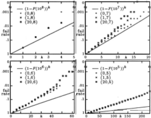
One property is the utility of the permanent trail­ markers learned. We tabulate the number of problems that require k memory accesses, and estimate A(k) by the fraction of problems unsolvable with the first k markers. To allow a closer look at the failure probabilities for large k, we plot the negative log of the failure frequencies in Figure 6, with reference line k log(1- P(.X)) anticipated by Theorem 1. For each algorithm, the data for k up to the size of the permanent memory is plotted. Several observations can be made from this figure. First, the ref­ erence lines do not approximate the (0, x) data very well , but do support all data from below. The bad approxima­ tion may be explained by the fact that the state space of the 15-puzzle is really not a random graph, but only an approximately regular graph. However, the appearance of the reference lines supporting the data from below provide evidence that the algorithms do perform more successfully than predicted under the idealized random­ graph model. Another observation is that as x decreases, A(l) becomes less trained than A(20). Simultaneously, the relative size of U(1) to that of U(20) also decreases, as indicated by the largest k attained for each data set. Obviously, as the power of local decreases (x decreases) , the more working markers is needed for faster bootstrap­ ping. With just one working marker, A(1) cannot learn as quickly as A(20) with thP- same number of training problems. Finally, we can clearly see the higher memory utility of A(1) compared to that of A(O), as predicted by Theorem 2. The data of type ( 1, x) is generally higher than that of type {0, x ). Although we do not see such generality between data of types {1, x) and {20, x ), we do also see that data of type (20, x) is generally higher than that of type of (0, x ). These data support our conjecture that EA(k)(m):::; EA(k)(O) for arbitrary m.

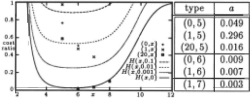
Finally, we measure the average search cost of each algorithm backed up by local( oo) and compare that with the theoretical predictions of Theorem 3. By straight­ forward computation, we have

where e!J+u~ 1 2 :::::: 6.43 x 10 8 is the theoretical average cost of local( oo ). Similarly,

giving us the upper bound of

for the ratio of the average search cost of A(m) backed up by local( oo) to that of local( oo) alone. We plot the theoretical upper bound for a = 0.1, 0.01, 0.001, 0, and the observed data points in Figure 7. The data points with observed failure probability a > 0 are listed in the adjacent table. Careful checking shows that the observed data points are indeed consistently lower than the pre­ dicted upper bound. Taking the failure probabilities into consideration, we see that A(20) with local{10 6 ) is the best of the 12 algorithms compared, yielding the lowest search cost ratio of 0.0159.

Now suppose that the upper bounds are indeed true. Then from H(x, 0), we see that after A(m) becomes fully trained (i.e., without the need of local( oo) as a backup), it can search with average cost less than that of local( oo) as long as x ~ 3, or c ~ 1000. However, from H(x, a) for a> 0, we see that if A(m) is not fully trained, then the range of x for which A(m) (with local(oo) as a backup) can search with average cost less than of local( oo) alone necessarily has an upper bound. For example, if a = 0.1, then x must be greater than 3.8 and less than 8.2. This 'over-learning' phenomenon of powerful local search becoming detrimental can be explained: If a > 0, then there may be problems more difficult than A(m) can handle; in this case, fruitless search will be incurred by A(m), causing local(oo) alone to be better.

6 Conclusion

We have presented an algorithm for bootstrap search, and provided some initial theory on their performance. Our theoretical analysis is based on a problem model of a random digraph. Using this model, we have made some strong performance predictions and comparisons of the algorithm. Further, we have illustrated some techniques for locating the optimal 'power' of the local search to be bootstrapped so as to yield the best global search. We have empirically evaluated our algorithm by applying it to both the 15-puzzle and a simple robot path planning problem. In both domains, we have 1) explained the observed performance behavior in terms of the theory developed; 2) explored the importance of having suffi­ ciently large set of working trail-markers; and 3) identi­ fied a common detrimental phenomenon of over-learning when local search becomes too powerful. Incidentally, we have also contributed some new results on solving the 15puzzle. In particular, we have made a natural but not widely recognized connection between search costs and the lognormal distribution.

Our work is by no means complete. Theoretically, we have not addressed the issue of training time, nor the issue of solution quality. Within the random digraph model, there are conjectures yet to be settled. Out­ side the random digraph model, there are plenty of other problem models that may yield further insights into the area of bootstrap search. In particular, the path plan­ ning problem addressed in this paper should provide mo­ tivation for a different model suitable for analysis. There may also be some other bootstrapping algorithms wait­ ing to be discovered. With its broad applicability in search and learning, further research is definitely needed.

A Proofs

Proof (Theorem 1) Since only A(O) is involved and c is constant, we drop parameter (0) and let F(c) = 1-a = a for notational simplicity. We first evaluate E(L(k) I A(k))· If R(U(k)) \ u(k) =f 0, then Uk+J can be found and whatever problems not in R(U(k)) will be reducible to Uk+l with independent probability a. However, if R(U(k)) \ U(k) is in fact empty, then (k) = oo and L(k) = 0. Th1s event can occur for k > 0 and with probability at most a(N-k+J)k when all N- k + 1 problems outside U(k) are not reducible to U(k)· (The first trail-marker that records the goal states is not considered part of the N problems.) Hence,

implying

which yields the desired result .

I

Proof (Theorem 2) (Sketch) Let the problem set be of finite size N; for infinite set, simply take the ap­ propriate limits. Let 0 ~ a, b ~ 1 be integral multiples of 1/ N. The proof of (2) is by induction on k; the base case of k = 0 is trivial. Given a particular digraph, we have

as a result of A(k+l)(m) = A(k)(m)-L(k)(m). Averaging over the digraphs and using the fact that the problems are uniformly distributed, we have

where PL(k, m, a, b) denotes the conditional average of Pr(L(k)(m) ~a- b) given that R(U(k)(m)) is some par­ ticular problem set X of size N(1- a). We now use two properties of PL whose proofs are more involved and are omitted:

From (14), we have

where ~PL(k, -1, a, b)= PL(k, -1, a, b)- PL(k, -1, a+ 1/N, b) is nonnegative from (15). Hence, by induction, we have

EPr(A(k+l)(1) ~b)

The induction step of showing

is done similarly. Finally, (3) follows directly from (2) and the fact that NEA(k )(m) = La EPr(A(!:)(m) > a)= L::a(l- EPr(A(k)(m) ~a)). I

Proof (Theorem 3) Let U[k] be the first k marker to be accessed. Let x be some problem, and K be the expected number of memory accesses before solving x or exhausting all available markers. Then

If the (k + 1)th entry exists and x is not in U[k + 1], then x will be in R~U[k + 1]) \ R(U[k]) with proba­ bility F(c)(1- F(c)) ; otherwise, x will not . Conse­ quently, K ~ Lk>o(k + 1)F(c)(1 - F(c))k = 1/ F(c). Thus, 'Y(c) ~ c(K-l)+'Yo(c) yields (4). If A(m) is backed up by local(oo), then the expected cost to be incurred by local( oo) can be at most the weighted cost of the most costly problems whose probability is a. Thus, f(c) ~ 'Y(c) + f;_ 1 (l-a) z dF(z) = 'Y(c) + 'Yo(oo)- 'Y1(1- a) . I