Possibility Theory as a Basis for Qualitative Decision Theory

1 Introduction

Standard approaches to decision under uncertainty are based on maximum expected utility theory. The expected utility criterion is particularly appealing since it can be justified on the basis of an axiomatic approach [von Neumann & Morgenstern, 1944]. However, its application requires that both numerical probabilities and utilities about the consequences of actions are available. The representation of incomplete states of knowledge has led Artificial Intelligence to introduce non-probabilistic models of uncertainty such as Shafer's theory of evidence, possibility theory, and nonmonotonic logics. These approaches seem particularly suitable for the representation of states of partial ignorance in an unbiased way; see [Dubois et al., 1994c] for a discussion. On the basis of a careful distinction between reasoning tasks (where consequences of the actual state of information are only propagated) and decision tasks (where choices are elaborated taking into account both uncertainty and preferences), it can be advocated that the probabilistic approach can still be used at the decision level even if another framework is used for knowledge representation and reasoning purposes; thus Smets [1990] has proposed a so­ called "pignistic" transformation for computing meaningful probabilities (in a decision-theoretic perspective) from belief functions representing the available information.

Possibility theory provides a faithful representation of par­ tial ignorance, but its core is also qualitative in nature since there exists a linear (i.e., complete partial) ordering~ over C expressing preference. Thus, a given act induces a preference over X, whereby x2':y iff f(x)2':f(y). This preference relation between precisely-known situations will be extended to in­ complete belief states pervaded with uncertainty by means of a relation obeying a series of axioms given in the following.

Indeed, we may have incomplete information about the actual situation in X. The belief state about which situation in X is the actual one is supposed to be represented by a possibility distribution 1t. A possibility distribution 1t defined on X takes its values on a valuation scale V, where V is supposed to be linearly ordered. V is assumed to be bounded and we take supV=l and infV=O. The inequality 7t(x)~7t(x') means that x' is at least as plausible (normal) as x as being the actual situation. 7t(x)=O means that x is impossible, i.e., definitely excluded by 1t as being the true situation. 7t(x)=l means that xis normal, unsurprizing. We restrict ourselves to consistent belief states 1t which are such that 3xE X, 7t(x)=l (i.e., there exists at least one situation which is completely possible); how this closely relates to the notion of logical consistency can be fully understood in the framework of possibilistic logic (e.g., [Dubois et al., 1994b, c]). The state of total ignorance 1t? is represented by V x E X, 7t 7 (x)= 1 where any situation is found totally possible. We shall denote by Pi(X) = { 1t, X~ V} the set of consistent possibility distributions over X. The cardinality of V is supposed to be at least as large as the one of X, so as to account for total plausibility orderings on X. Clearly, X~Pi(X) using the identification function xo~ll{xo} where 7t(x)=lltxo}(x)= 1 if x=xo and ll{xol (x)=O otherwise. ll{xo} is called a precise belief state and we shall write, 7t={x0}, or even 7t=xo for the sake of notational simplicity. More generally, if 1t is the characteristic function of a subset A of X, we write 7t=A. For instance 1t? = X.

A possibility distribution representing a belief state involves a set of mutually exclusive alternatives, where each element can be ranked according to its level of plausibility to be the true situation. Let x C)nd y be two elements of X, the possibility distribution 1t defined by 7t(x)=A, 7t(y)=j1., 7t(z)=0 for z:;t:x, z:;t:y with max(A,jl.)=l (in order to have 1t normalized), will be called a qualitative lottery and will be denoted by (A./x, jl./y), which means that we are either in situation x or in situation y with the respective levels of possibility A. and ll· More generally, any possibility distribution 1t can be viewed as a multiple-consequence lottery (A.11x1, .. . ,A.n/xn) where X={x1, .. . ,xnl and Aj=1t(Xj). We will also use the notation (A./1t 1, j1./1t2) (with max(A,jl.)= 1) for denoting the compound possibility distribution 7t= max(min(7t 1 ,A),min(7t 2 ,j1.)). This can be viewed as a lottery over multiple-consequence lotteries corresponding to 1t1 and 1t 2 . The lottery (A/x, jl./y) can be viewed as a particular case of it when 1t1 and 1t2 are possibility distributions focusing on singletons. The resulting possibility distribution 7t= max(min(7t 1 ,A.),min(7t2,jl.)), with max(A,jl.)= I, is here the qualitative counterpart of probabilistic mixtures A.p 1 +(l­ A.)p2; see [Dubois & Prade, 1990], [Dubois et al., 1993].

Lastly, the decision maker (DM) is supposed to express a preference between (consistent) belief states. This preference relation, denoted by l:;, should be understood in the following way: 7tl:; 1t' means that DM expects at least as much in terms of pay-off when he believes 1t than when be believes 1t'. We suppose that Axiom 1: l:; is a complete partial ordering.

>- shall denote the strict relation associated with l:;, and 1t ~ 1t' will mean that 7tl:; 1t' and 7t'C.,7t. A qualitative utility function is a mapping u from Pi(X) to a linearly ordered scale U. Thus, u(1t) will denote the ordinal evaluation of an act in the state of belief 1t. We shall simply write u(x) (instead of u({x}), when 7t={x}, for denoting the utility of the considered act when the situation is precisely known as being x. We also write u(A) instead of u(1t) with 7t=llA (characteristic function of subset A). As usual, a (qualitative) utility function u will be said to represent a preference ordering l:: if and only if u(7t)~u(7t')<=>7tl:;7t'.

Together with Axiom I, we propose the following axioms as a basis of our decision theory.

Axiom 2 (certainty equivalence): If the belief state is a crisp set A~X. then there is xE A such that { x} ~A.

The intuition behind Axiom 2 is the following one. The decision-maker DM only knows that one of the situations in A is the true situation. Hence, the utility of the act should lie in the set { u(x), XE A}, where u(x) is the utility of the act in situation x. The choice of the state x such that u(x)=u(A) reflects DM's attitude towards risk.

Axiom 3 (risk aversion, or "precision is safer"): 1t~7t' ~ 1tl:; 1t' .

The motivation underlying this axiom is that DM prefers the belief state which are more precise. Indeed if 1t~1t' (i .e., 'VxE X, 7t(x)~7t'(x)), it means that belief state 1t' is less informed than belief state 1t (since according to 1t' any situation x is found to be at least as much possible as according to 7t). Thus, 1t' is viewed as a more risky belief state than 1t, since the worst situation pertaining to 1t' is not less possible than the worst situation pertaining to 1t. Behaving in this way DM is cautious. This is a risk-averse attitude since, for all x in A {x}l:;A, i.e., in terms of a utility function u(x)~u(A) . This means that DM prefers to be in situation x for sure, than only knowing that he is in A and having the possibility of receiving less, in case 3yE A and u(y)<u(x). Total ignorance is always the worst situation. At this point, it should be clear that the utility function we look for is in accordance with Wald maximin criterion.

It is assumed that max(A,jl.)= I in order to ensure that the new possibility distributions built from 1t1, 1t2, 1t' are still normalized. Axiom 4 means that if two belief states are judged to be equivalent from a pay-off point of view, this equivalence still holds when we substitute one of these belief states by the other in compound lotteries, thus expressing a form of independence. Indeed this axiom is a possibilistic counterpart of the so-called linearity or independence axiom in von Neumann & Morgenstern' utility theory.

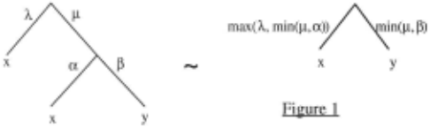
Axiom 5 (reduction of lotteries):

This axiom reduces meta lotteries to ordinary ones. Again it is assumed that max(A,jl)=1=max(a,p) in order to guarantee normalization preservation. This axiom, which is the counterpart of von Neumann & Morgenstern' substitutability axiom, can be better understood by visualizing what it expresses in terms of qualitative lotteries, as shown on Figure 1. Namely, if two steps are needed to reach situation y, one which succeeds with possibility jl, and the next one that succeeds with possibility p, then the possibility of reaching situation y is not higher than min(jl,p). However, if alternative paths exist, leading to x, with respective possibility levels A and jl, then the possibility of reaching x is at least max(A,jl).

This axiom is reminding of continuity axioms in classical utility theory. (1/1t,A/X) is a meta-lottery whereby it is slightly possible to be in a state of total ignorance instead of in belief state 1t. Clearly, the lottery (1/1t,A/X) corresponds to the possibility distribution 7t"=max(1t,A) and is a state of belief less informed than 1t. When A=l 1t"=1t? and we know by Axiom 3 that u(1t7):S:u(1t), \f1tE Pi(X). Moving A in V from 0 to 1, when 1tC,1t', leads to decrease the preference down to a possibility distribution which is not preferred to 1t'. The idea behind Axiom 6 is that 1t' is hit for some value of A.

3 Form of the Qualitative Utility Function

Theorem: Given a preference relation C. on Pi(X) verifying Axioms 1 to 6, there exists a fuzzy set F on X and a utility function u from Pi(X) to a totally ordered set U representing c. such that for each 1tE Pi(X), we have

where n is an order reversing function from the possibility scale V to the preference scale U such that n(O)=l and n(l)=O where 1 denotes the top elements of U and V and 0 their bottom elements.

Note that (1) yields u(x)=!lp(x).

Proof:

I) u defined by ( 1) satisfies Axioms 1 to 6. This is obvious for Axioms 1, 3 and 4 Axiom 2: If 1t=llA· \fxE A, n(1t(x))=O and \fx~ A,

n(1t(x))= 1. Thus u(1t)=minxE A u(x) and then 3xE A, u(1t)=u(x). Note that 1t? is such that u(1t? )=min7tE Pi(X) u(1t)=infxE X u(x).

Axiom 5: Note that

u((A/x, !lfy)) = min(max(u(x),n(A)),max(u(y),n(Jl))) and that

u((Af1t1, !lf1t2)) = u(max(min(1tt ,A),min(1t2,11)))

• =minx max(n(max(min(1t1 (x),A),min(1t2(x),!l)),u(x))

=minx max[min(max(n(1t1 (x)),n(A.)), .

max(n(1t 2 (x) ),n(jl)) ),u(x)]

=minx min(max(n(1t 1 (x)),u(x),n(A)),

max(n(1t2(x)),u(x),n(!l)))

= min(max(u(1t1 ),n(A)), max(u(1t2),n(jl))).

Then, it can be easily checked that

u((A/x, !lf(alx, Ply))

= min(max(u(x),n(A.)),max(u((a/x, Pfy)),n(jl)))

= min(max(u(x),n(A)),max(min(max(u(x),n(a)),

max(u(y),n(P)),n(jl)))

• = min(max(u(x),min(n(A),max(n(jl),n(a)))), max( u(y ),n(jl),n(P)))

= min(max(u(x), n(max(A,min(jl,a))),

max(u(y),n(min(jl,p))))

= u((max(A,min(jl,a))/x,min(jl,p)/y).

Axiom 6: u(1t)~u(1t'). Let A.=n-l(u(1t')). Then u(l/1t,A.IX) = min(u(1t),max(u(1t'),u(1t 7 )) = u(1t').

Remark: Note that we have the following consequence: 1t~1t' ~ 1t~max(1t,1t').

It means that if two belief states are considered as equally risky, it is indifferent for the DM to be in any of these belief states. For instance, it { x} ~ { x'}, then the DM does not wish to know whether the situation is x or x' since his pay-off will be the same in both cases; hence we shall have u({x,x'})=u(x)=u(x').

Indeed the form (2) of the utility function leads to: u(max(1t,1t'))= min(u(1t),u(1t'))=u(1t)=u(1t').

• II) Existence of a utility function u of the form ( 1 ), given Pi( X) equipped with~.

First, consider the restriction of (Pi(X), c) to (X,c.). Let us map (X,c.) to an ordinal scale U such that inf(X) is mapped to 0 and sup(X) is mapped to 1.

Let u be a function from X to U such that u(x)~u(y) ~ xc.y. The proof then goes as follows:

1. extension of the utility function from X to its power set 2X. This enables us to compare states of incomplete information;
2. definition of the utility of the elementary lottery (1/supX, AlinfX) (or equivalently (111, A/0) since by definition u(supX)=l and u(infX)=O), for any AEV;
3. computation of the utility of the qualitative lottery (1/x, A/y) for any x, yE X;
4. prove that u((l/1t, 111t'))=min(u(1t),u(1t'));
5. computation of u(1t) for any state 1t of incomplete information.
6. Function u can be extended to subsets A of X in the following way u(A)=minxE A u(x). Indeed, if xA ~A, where xA E A, is the certainty equivalent of A (according to Axiom 2), then \fxEA, xc.xA. This can be easily shown in the following way. Assume 3xE A, xA>-x; then by Axiom 3, xA>-X!::.A (since ll{x}:S:JlA), hence

(2)

xA>-A which contradicts the hypothesis. Hence u(A)= u(xA)=minxEA u(x).

Note that A denotes a state of information where the consequence of the act under evaluation is only known to lie in A. u(A) is thus the pessimistic utility criterion proposed by Wald when the probability of outcomes in A are not available.

b) Let x=infX such that u(x)=O and x=supX, such that u(x)=l. Consider AE V a level of possibility, and the lottery (1/x, A./x). Let n be a bijection v~u such that \fu 1 ,u2E V, UJ <u2 ~ n(uJ)>n(u2), n(O)=l, n(l)=O.

Then Jet us define u(l/x, A./x)=n(A.). This definition agrees with any preference ordering~ on Pi(X). Indeed

(as shown in a)) and n(l)=O=u(x).

Moreover Axiom 3 enforces (1/x, A./x)dl/x, A.'/x) whenever A.~A.' (since the lottery (1/x,A./x.) is more informed than the other), and we do have that u(l/x, A.!x_)?. u(l/x, A.'/x_). Hence the definition of the qualitative utility is in agreement with the axioms. It is clearly a special case of (I) for 1t(x)= l if x= X:, A. if x=x, and 0 otherwise, and JlF(x)=u(x).

c) Now consider the lottery (1/x, A./y) for x, yE X.

· Assume first that u(x)~u(y). Let us prove that u( 1/x,

A./y)=u(x). Indeed

(1/x, A./y) ~ (x,y} (Axiom 3)

{x,y} ~x

(Axiom 2)

x ~ (1/x, A./y)

(Axiom 3)

hence (1/x, A./y) ~ x and they have the same utility values.

• Assume now that u(x)?.u(y). First note that y~(llx, n-I(u(y))/x.). Indeed u(y)=no n-l(u(y)) by definition. If x=x, then

(independence Axiom 4)

Hence u(l/x, A./y) = n(max(n-l(u(y),A.)) = min(u(y),n(A.)).

• In the general case, if x?.y then y~ (llx, Jl!X) (Axiom 6) for some JlE V and since X contains x (at worst x=y), X~x.. Hence, using the independence Axiom 4, y~ (1/x, Jllx.). Now we note that x~ (llx, n-1(u(x))/x), and we can substitute:

• "' (1/x, max(n-l(u(x)), Jl), x) using Axiom 5 on the lottery below

Hence u(y)=min(u(x),n(Jl))=n(Jl) since x?.y. Hence Jl= n-l(u(y)). So y~ (l/x,n-l(u(y))/x) (note the presence of X, and no longer X).

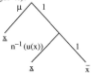
min(A., n-l(u(y))/x) (Axiom 5) Hence u(l/x, A./y)=min(u(x),max(n(A.),u(y))) when it is thus valid regardless of the preference on { x,y} .

x?.y. Note that if x~y. the above expression yields u(x); d) Consider two possibility distributions 1t, 1t' with 1t?.

1t'. Then from Axiom 6, 3A.EV, 1t'~ (I/1t,A./X) , hence

Hence u(max(1t,1t'))=u(1t') when u(1t')~u(1t), noticing that the lottery (1/1t, 1/1t') encodes the possibility distribution max(1t,1t').

e) Lastly we can compute u(1t) for any 1tE Pi(X). Let 1tE Pi(X), and assume that 1t(xl)=l?.1t(x2)?. ... ?.1t(xn) . Let 1tjE Pi(X) be such that 1tj(x 1 )=1, 1tj(Xj)=1t(xj). and 1tj(x)=0 if xE: {x1,xj}. Then 1t~ (l11tJ,l/1t2 , . .. ,l/1tn) , since 1t=maxi=l ,n 1ti . Hence u(1t)=mini=l ,n u(1tj) from d) . Now u(1tj)=min(u(x 1 ),max(n(1t(xi)),u(xj))) from c). Hence

u(1t) =mini= I ,n min(u(x 1 ),max(n(1t(x 1 )),u(x 1)))

= mini=l,n max(n(1t(Xj)),u(xj)) noticing that 1t(x 1 )=1. The fuzzy set F is such that !J.F(x)=u(x), VxE X.

4 Properties of the Qualitative Expected Utility

Interestingly enough the qualitative utility introduced in the previous section, u(1t)=minxE x max(n(1t(x)) ,u(x)) is the necessity of a fuzzy event [Dubois & Prade, 1980] in the sense of possibility theory, namely u(1t)=N1t(F) where F is the fuzzy set of preferred situations (JlF(x)=u(x) , VxE X) and N1t is the necessity measure based on the possibility distribution 1t. Usually, when V =U=[O, 1 ], n(t)=l-t in the above expression. N1t(F) can be viewed as a degree of inclusion of the fuzzy set of more or less possible situations in the fuzzy set F of preferred outcomes, i.e. , it estimates the certainty that the belief state 1t corresponds to the preferred situations described by F. As already said, there is a commensurability assumption made between the uncertainty scale and the preference scale, since possibility degrees and utility degrees are aggregated in the expression of u(1t). Note that

• N1t(F)=u(1t)=l iff {xEX, 1t(x)>0} ~ {xEX, u(x)=l}

i.e., the utility of 1t is maximum if all the more or less possible situations encompassed by 1t are among the most preferred ones.

• N1t(F)=u(1t)=O iff { XE X, 1t(x)=1 } n { xE X, u(x)=O }#0 i.e., the utility of 1t is minimum if there is one of the most plausible situations whose pay-off is minimum (we recognize the risk-aversion of the approach). N1t(F)=u(1t) is all the greater as there is no situations with a high

plausibility and low utility value.

When 1t is the characteristic function of an ordinary subset A of X, i.e., when all the situations encompassed by the belief state are equally plausible, as already said the utility u(1t) simplifies into u(1t)=minxE A u(x) where we recognize Wald [1950]'s pessimistic criterion which leads to decisions maximizing the minimal pay-off. In the general case, u(1t) takes into account the fact that all the situations are not equally plausible in the set { xE X, 1t(x)>0}.

Several authors have proposed definitions of utility functions in the presence of possibilistic uncertainty, including the form described in the theorem. Yager [1979] has introduced the possibilistic extension of the optimistic maximax criterion of the form dual to (1), i.e., u(1t)= maxxE x min(1t(x),!J-p(x)) which is the degree of possibility of a fuzzy set [Zadeh, 1978]. The possibilistic counterpart of Wald maximin criterion of the form proposed here, has been introduced by Whalen [1984], in terms of "disutility" function D(1t)=n-l(u(1t)) where u(1t) is given by (1). D(1t) takes the form of the degree of possibility of the fuzzy set F (the fuzzy complement of F) of less preferred situations.

As already pointed out (e.g., [Inuiguchi et al., 1989]), the expression of the necessity of a fuzzy event is a particular case of a fuzzy integral in the sense of Sugeno [1974]. Namely Nn(F) can be shown to be equal to (for V= U=[0,1])

with Fa={xEX, !J-p(x)~a}, which is a particular case of Sugeno integral

with Ha={ XE X, h(x)~a} and g is a set function monotonic with respect to set inclusion, such that g(0)=0 and g(X)=l. Sugeno integrals can be regarded as qualitative counterparts I to Choquet integrals of the form J g(Ha)da. Sugeno 0 integrals in general have been recently considered by Hougaard & Keiding [1994] for the utility representation of preferences on the set of non-additive set functions.

The utility function advocated in this paper relies on the notion of possibilistic mixture (as it can be seen in particular in Axiom 5), the result of the possibilistic mixture of n 1 and n2, with max(a,P)=1, being equal to 1t= max(min(n1 ,a),min(1t2,p)). Namely if fli is a possibility measure such that for all events A, B, ITi(AuB)= max(flj(A),flj(B)), then max(min(IT1 ,a),minCIT2,p)) is again a possibility measure; see Dubois & Prade [1990]. This is a particular case of extended mixtures of decompo­ sable measures (which are a family of set functions encom­ passing probability measures and necessity and possibility measures as particular cases), as studied in [Dubois et al., 1993] where application to utility theory is pointed out.

Lastly, it should be emphasized that the proposed approach to qualitative utility closely parallels von Neumann & Morgenstern' theory and that there is some similarity between the two sets of axioms underlying the two approaches. Clearly, there are other ways of "distorting" classical utility theory. For instance, one of the authors

[Dubois, 1986] has relaxed the reduction of lotteries axiom in a purely probabilistic framework by using a special family of operators in place of multiplication for expressing a relaxation of probabilistic independence. We might also think of using the multiplication instead of the min operation when simplifying numerical possibilistic lotteries, i.e., using mixtures of the form max(a-n1, P·n2) with max(a,P)=l. This would lead to a utility function of the form u(1t)=minxEX [1-(1-u(x))·1t(x)].

5 Handling Uncertainty in Flexible Constraint Satisfaction Problems

A constraint satisfaction problem is defined as a set V= { v 1, ... , v n} of decision variables, where Di is the range of vi, for all i, and a set of constraints {C1, ... ,Cml· Each constraint Cj refers to a relation Rj that links a subset Vj~V of variables, i.e., Rj is a subset of the Cartesian product xv·EV· Di, such that the restriction (v1, ... ,vn)J.y. of I J J ( v 1, ... , v n) to the variables in Vj should belong to Rj for all constraints c1, ... ,Cm. The constraint satisfaction problem consists in finding a feasible solution ( d 1, ... ,dn) to the set of constraints {C1, ... ,Cml·

A flexible constraint is a constraint that can be violated to some extent. A flexible constraint can be modelled as a set of ordinary relations R l ... Rk, such that R l~R2~ ... ~Rk. Namely R2 is a relaxation of R l, R3 is a relaxation of R2, etc. [Freuder, 1989]. An equivalent modelling consists in viewing a flexible constraint as a fuzzy relation m, where !J-R ( d 1, ... ,dn) is the degree of satisfaction of solution ( d 1, ... , dn) [Zadeh, 197 5]. The two views are equivalent if we attach satisfaction weights uj, j=1,k to Rj such that u 1 =1~u2~- - -~ uk>O, all weights belonging to a totally ordered scale U. Then define !J-R(d1, ... ,dn) as follows !J-R(dl, ... ,dn)=max{ui, (d1 , ... ,dn)E Ri }. Conversely Ri={ (dJ , ... ,dn),!J-R(d1 , ... ,dn)~ uil· It is possible to view the set {Rl, ... ,Rk) ask prioritized constraints, where Rj has a higher priority than Ri when j<i [Dubois et al., 1994a].

It often happens that uncertain parameters are involved in constraint satisfaction problems. For instance, in scheduling problems, the starting time of an activity is controlable and is a decision variable, but the ending time of the activity is partially unknown even if the starting time has been decided and is known, because the duration of the activity is partially uncontrollable. If there is a flexible constraint on the ending time of the activity, the degree of satisfaction of the decision consisting in the choice of a starting time is not precisely known. Let z1, ... ,zp be a set of uncertain parameters involved in a constraint satisfaction problem. A constraint C (a flexible one, generally) relates decision variables v 1, ... , v n and uncertain parameters z 1, ... ,zp. Let Ek the domain of zk. Then the lack of knowledge on the parameter zk is modelled by a possibility distribution 7tk, and the possibility distribution 1t attached to (zl, ... ,zp) is 1t=mink=l,p 1tk [Dubois & Prade, 1988]. Let z=(z1 , ... ,zp) and d=(d1 , ... ,dn)· The degree of satisfaction of C by (d,z) is J.!R(d,z) and is ill-known, because so is z. A robust solution to the constraint C is d such that (d,z) satisfies C for all possible values of z.

In the non-flexible case, and assuming that the possible values of z form a subset A of E1 x .. . xEP, v=d is a robust solution to constraint C if and only if VzE A, (d,z)E R that is, dER(v)={d,{d}xA~}.

In the general case Jet A I ={z,7t(z)= 1 } be the set of normal values of z and A be the set of possible values of z (i.e., no value is possible outside A). Similarly let R I be the set of preferred values of (v,z) and B. be the set of feasible values of (v,z). Then a completely robust solution dis one that totally satisfies C for all possible values of Z, i.e.,

A partially robust solution d is one that partially satisfies C for all normal values of z, i.e. ,

The qualitative utility function enables a degree to which d is a robust solution to C to be computed as follows

Accepting a solution such that Jlc(d)~a. where aE U, means that

• one accepts to assume that the actual value of z will lie in A n(a)= { zln(z)~n( a)} where n is the order-reversing function that maps degrees of preference aE U to degrees of possibility in V ;
• taking this assumption for granted, any solution such that Jlc(d)~a satisfies for sure the constraint C to level a for any eventual value of z in An( a).

Again, the qualitative utility function tries to compromise between uncertainty and preference via a commensurateness assumption. A solution is all the better if it can cope with more implausible values of uncertain parameters.

Example: Tom wants to attend a meeting that starts at eight o'clock, and wants to decide when to get up so as to arrive on time. He has to take a bus, and the ride takes about 1 hour. He does not want to leave his home too early, say before 7 but not before 6.30. This is modelled by a fuzzy interval M such that M=[6.5, 7] and M'={7}. The constraint on the arrival time is that not more than 114 hour delay is acceptable, so that it is a fuzzy interval N with Nl=[7, 8] and N=[7, 8.25]. The uncertainty about the trip duration is modelled by a possibility distribution 7t=J.!A with A 1 = { 1 } and A=[0.75, 1.25] because if Tom is lucky (no wait, no traffic) the trip takes 3/4 hour, while if he is unlucky, it may take l/2 hour more. The problem is to find a starting time s for the trip, such that s lies in M (constraint about getting up), and so that whatever the duration z of the trip the arrival time s+z is acceptable, i.e., lies in N. Applying the above qualitative utility theory with U=V=[O,l], and n(a)=1-a, it comes down to finding s which maximizes min(J.!M(s), infz max(1-J.!A(z),J.!N(s+z)) where J.!M, J.!A, J.!N are membership functions. To understand this expression, it is enough to see it as a multiple-valued evaluation of the sentence 3s, sE M and Vz if ZE A then S+tE N. The maximization and the minimization are multiple-valued counterparts of the universal and the existential quantifiers respectively, and max(l-a,b) is a multiple-valued implication. The term infz (max( 1-J.!A (z),J.!N(s+z)) is the qualitative utility of choosing s as a starting time decision, in a situation where the incomplete knowledge about z is defined by 7t=J.!A, and where the preference level of decisions in situation z is J.!p(z)=J.!N(s+z) (evaluating to what extent the arrival time constraint is violated). With linear member­ ship functions it is found that Tom should leave his home at 6:52'30" am; then provided that the trip does not exceed I: 11 '20", it ensures that Tom will not be more than 3'50" late. Note that the trip length estimate is rather safe. See Dubois et a!. [ 1995] for a full treatment of this example, and the application of this approach to job-shop scheduling.

6 Decision with Generic Knowledge and Generic Preference Information

Belief states are often incompletely specified through the use of pieces of knowledge and information, some of which being uncertain. In other words, a possibility distribution over the possible situations is not always explicitly specified. Besides, preferences might also be incompletely specified. An instance of such problems is given by the following motivating example used in [Tan & Pearl, 1994b] and Boutilier [1994]. An agent is supposed i) to know that "if I have the umbrella, then I will be dry", u~d; "if it rains and I do not have the umbrella, then I will be wet", rA-.u~-.d; and "typically if it is cloudy, it will rain", c~r. (the latter rule is uncertain) ii) to observe that the sky is cloudy, iii) to prefer being dry rather being not dry d>--.d and carrying no umbrella -.u>- u. It is further assumed that "being dry is more important than not carrying an umbrella" (d>--.u). The problem is then for the agent to decide whether or not to take an umbrella.

Interpreting rules via material implication, knowledge expressed by (i) can be encoded in possibilistic logic [Dubois et al., 1994b] by assuming N(-.uvd)= 1, N(-.rvuv-.d)=l, N(-.cvr)=1-A<1 and N(c)=l, where N is a necessity measure. The least informative possibility distri­ bution (on interpretations) obeying these constraints is such that the situations rAU/\d and rA-.uA-.d have possibility I, -.r/\U/\d and -.r/\-.u/\d and -.r/\ -.u/\-.d have a smaller possibility, say A, with O<A<l, while the other situations are virtually impossible. Note that the precise value of level A remains unknown in our example. We have also to define the fuzzy sets of preferences Fu and F -.u· associated with the actions 'taking an umbrella' and 'not taking an umbrella', over the set of relevant situations. Fu will be a nonnormalized fuzzy set (Jlfr/\U/\d, J.!l-.r/\UAd) with J.!<1 caused by agent's reluctance to carry an umbrella. F -.u will be the fuzzy set (a/rA-.uA-.d, 13/-.r/\-.u/\ d, ahr/\-.uA-.d) with 13>a. Moreover, a<Jl since it is more important to be dry than not to carry an umbrella. It can be checked that

Nn(F u)=min(Jl,max(J.!,n(A) )=Jl

and Nn(F -.u)=min( a,max(n(A),I3 ),max(n(A),a)=a<Nn(F u). It leads to the decision: "take an umbrella". The value of A does not influence the result since the important point in this very elementary example is that it is strictly more plausible that it rains rather than it does not rain, and our approach is risk-averse (that is, here, rain-averse). Note that in the above example, the rules are not conflicting. In the case of conflicting rules one may use the method developed by Benferhat eta!. [1992] for encoding exception-prone rules in possibilistic logic.

7 Concluding Remarks

We have proposed a utility-based, axiomatically-grounded, decision theory which only requires ordinal scales for the assessment of uncertainty and preferences. The proposed approach opens the road to a genuine decision theory in the framework of possibility theory, a long term goal which was already at the basis of the work of the English econo­ mist Shackle [1961]. It can be applied in problems where the information is very rough and qualitative, including decision-theoretic planning. If we can afford scales with a somewhat richer structure, we may, for instance, as suggested at the end of Section 4, use a product-based rather than a min-based approach. Due to the equivalence between "max-product" possibility theory and Spohn [1988]'s ordinal conditional "kappa" functions up to a rescaling (see [Dubois & Prade, 1991 ]), it would lead to a decision-theoretic framework for kappa functions , whose axiomatization could be investigated both in the possibilistic setting and in the von Neumann-Morgenstern framework (with infinitesimal lotteries). This is a topic for further research.